VOLUME VIII SLICE IV Diameter to Dinarchus (continued 8)

Consider, in fact, a single infinity of connected elements each satisfying F = 0, say a chain connectivity T, consisting of elements specified by x0, y0, z0, p0, q0, which we suppose expressed as Complete integral constructed with characteristic chains. functions of a parameter u, so that

U0 = dz0/du − p0dx0/du − q0dy0/du

is everywhere zero on this chain; further, suppose that each of F, dF/dp, ... , dF/dx + pdF/dz is developable about each element of this chain T, and that T is not a characteristic chain. Then consider the aggregate of the characteristic chains issuing from all the elements of T. The ∞² elements, consisting of the aggregate of these characteristic chains, satisfy F = 0, provided the chain connectivity T consists of elements satisfying F = 0; for each characteristic chain satisfies dF = 0. It can be shown that these chains are connected; in other words, that if x, y, z, p, q, be any element of one of these characteristic chains, not only is

dz/dt − pdx/dt − qdy/dt = 0,

as we know, but also U = dz/du − pdx/du − qdy/du is also zero. For we have

dU = d ( dz − p dx − q dy ) − d ( dz − p dx − q dy )

dt dt du du du du dt dt dt

= dp dx − dp dx + dq dy − dq dy ,

du dt dt du du dt dt du

which is equal to

dp dF + dx ( dF + p dF ) + dq dF + dy ( dF + q dF ) = − dF U.

du dp du dx dz du dq du dy dz dz

As dF/dz is a developable function of t, this, giving

U = U0 exp( − ∫ t dF dt ),

t0 dz

shows that U is everywhere zero. Thus integrals of F = 0 are obtainable by considering the aggregate of characteristic chains issuing from arbitrary chain connectivities T satisfying F = 0; and such connectivities T are, it is seen at once, determinable without integration. Conversely, as such a chain connectivity T can be taken out from the elements of any given integral all possible integrals are obtainable in this way. For instance, an arbitrary curve in space, given by x0 = θ(u), y0 = φ(u), z0 = ψ(u), determines by the two equations F(x0, y0, z0, p0, q0) = 0, ψ′(u) = p0θ′(u) + q0φ′(u), such a chain connectivity T, through which there passes a perfectly definite integral of the equation F = 0. By taking ∞² initial chain connectivities T, as for instance by taking the curves x0 = θ, y0 = φ, z0 = ψ to be the ∞² curves upon an arbitrary surface, we thus obtain ∞² integrals, and so ∞4 elements satisfying F = 0. In general, if functions G, H, independent of F, be obtained, such that the equations F = 0, G = b, H = c represent an integral for all values of the constants b, c, these equations are said to constitute a complete integral. Then ∞4 elements satisfying F = 0 are known, and in fact every other form of integral can be obtained without further integrations.

In the foregoing discussion of the differential equations of a characteristic chain, the denominators dF/dp, ... may be supposed to be modified in form by means of F = 0 in any way conducive to a simple integration. In the immediately following explanation of ideas, however, we consider indifferently all equations F = constant; when a function of x, y, z, p, q is said to be zero, it is meant that this is so identically, not in virtue of F = 0; in other words, we consider the integration of F = a, where a is an arbitrary constant. In the theory of linear partial equations we have seen that the integration Operations necessary for integration of F = a. of the equations of the characteristic chains, from which, as has just been seen, that of the equation F = a follows at once, would be involved in completely integrating the single linear homogeneous partial differential equation of the first order [Fƒ] = 0 where the notation is that explained above under Contact Transformations. One obvious integral is ƒ = F. Putting F = a, where a is arbitrary, and eliminating one of the independent variables, we can reduce this equation [Fƒ] = 0 to one in four variables; and so on. Calling, then, the determination of a single integral of a single homogeneous partial differential equation of the first order in n independent variables, an operation of order n − 1, the characteristic chains, and therefore the most general integral of F = a, can be obtained by successive operations of orders 3, 2, 1. If, however, an integral of F = a be represented by F = a, G = b, H = c, where b and c are arbitrary constants, the expression of the fact that a characteristic chain of F = a satisfies dG = 0, gives [FG] = 0; similarly, [FH] = 0 and [GH] = 0, these three relations being identically true. Conversely, suppose that an integral G, independent of F, has been obtained of the equation [Fƒ] = 0, which is an operation of order three. Then it follows from the identity [ƒ[φψ]] + [φ[ψƒ]] + [ψ[ƒφ]] = dƒ/dz [ψφ] + dφ/dz [ψƒ] + dψ/dz [ƒφ] before remarked, by putting φ = F, ψ = G, and then [Fƒ] = A(ƒ), [Gƒ] = B(ƒ), that AB(ƒ) − BA(ƒ) = dF/dz B(ƒ) − dG/dz A(ƒ), so that the two linear equations [Fƒ] = 0, [Gƒ] = 0 form a complete system; as two integrals F, G are known, they have a common integral H, independent of F, G, determinable by an operation of order one only. The three functions F, G, H thus identically satisfy the relations [FG] = [GH] = [FH] = 0. The ∞² elements satisfying F = a, G = b, H = c, wherein a, b, c are assigned constants, can then be seen to constitute an integral of F = a. For the conditions that a characteristic chain of G = b issuing from an element satisfying F = a, G = b, H = c should consist only of elements satisfying these three equations are simply [FG] = 0, [GH] = 0. Thus, starting from an arbitrary element of (F = a, G = b, H = c), we can single out a connectivity of elements of (F = a, G = b, H = c) forming a characteristic chain of G = b; then the aggregate of the characteristic chains of F = a issuing from the elements of this characteristic chain of G = b will be a connectivity consisting only of elements of

(F = a, G = b, H = c),

and will therefore constitute an integral of F = a; further, it will include all elements of (F = a, G = b, H = c). This result follows also from a theorem given under Contact Transformations, which shows, moreover, that though the characteristic chains of F = a are not determined by the three equations F = a, G = b, H = c, no further integration is now necessary to find them. By this theorem, since identically [FG] = [GH] = [FH] = 0, we can find, by the solution of linear algebraic equations only, a non-vanishing function σ and two functions A, C, such that

dG − AdF − CdH = σ(dz − pdz − qdy);

thus all the elements satisfying F = a, G = b, H = c, satisfy dz = pdx + qdy and constitute a connectivity, which is therefore an integral of F = a. While, further, from the associated theorems, F, G, H, A, C are independent functions and [FC] = 0. Thus C may be taken to be the remaining integral independent of G, H, of the equation [Fƒ] = 0, whereby the characteristic chains are entirely determined.

When we consider the particular equation F = 0, neglecting the case when neither p nor q enters, and supposing p to enter, we may express p from F = 0 in terms of x, y, z, q, and then eliminate it from all other equations. Then instead of the equation [Fƒ] = 0, we have, if F = 0 give p = ψ(x, y, z, q), the equation

Σƒ = − ( dƒ + ψ dƒ ) + dψ ( dƒ + q dƒ ) − ( dψ + q dψ ) dƒ = 0,

dx dz dq dy dz dy dz dq

moreover obtainable by omitting the term in dƒ/dp in [p − ψ, ƒ] = 0. Let x0, y0, z0, q0, be values about which the coefficients in The single equation F = 0 and Pfaffian formulations. this equation are developable, and let ζ, η, ω be the principal solutions reducing respectively to z, y and q when x = x0. Then the equations p = ψ, ζ = z0, η = y0, ω = q0 represent a characteristic chain issuing from the element x0, y0, z0, ψ0, q0; we have seen that the aggregate of such chains issuing from the elements of an arbitrary chain satisfying

dz0 = p0dx0 − q0dy0 = 0

constitute an integral of the equation p = ψ. Let this arbitrary chain be taken so that x0 is constant; then the condition for initial values is only

dz0 − q0dy0 = 0,

and the elements of the integral constituted by the characteristic chains issuing therefrom satisfy

dζ − ωdη = 0.

Hence this equation involves dz − ψdx − qdy = 0, or we have

dz − ψdx − qdy = σ(dζ − ωdη),

where σ is not zero. Conversely, the integration of p = ψ is, essentially, the problem of writing the expression dz − ψdx − qdy in the form σ(dζ − ωdη), as must be possible (from what was said under Pfaffian Expressions).

To integrate a system of simultaneous equations of the first order X1 = a1, ... Xr = ar in n independent variables x1, ... xn and one dependent variable z, we write p1 for dz/dx1, &c., System of equations of the first order. and attempt to find n + 1 − r further functions Z, Xr+1 ... Xn, such that the equations Z = a, Xi = ai,(i = 1, ... n) involve dz − p1dx1 − ... − pndxn = 0. By an argument already given, the common integral, if existent, must be satisfied by the equations of the characteristic chains of any one equation Xi = ai; thus each of the expressions [XiXj] must vanish in virtue of the equations expressing the integral, and we may without loss of generality assume that each of the corresponding ½r(r − 1) expressions formed from the r given differential equations vanishes in virtue of these equations. The determination of the remaining n + 1 − r functions may, as before, be made to depend on characteristic chains, which in this case, however, are manifolds of r dimensions obtained by integrating the equations [X1ƒ] = 0, ... [Xrƒ] = 0; or having obtained one integral of this system other than X1, ... Xr, say Xr+1, we may consider the system [X1ƒ] = 0, ... [Xr+1ƒ] = 0, for which, again, we have a choice; and at any stage we may use Mayer’s method and reduce the simultaneous linear equations to one equation involving parameters; while if at any stage of the process we find some but not all of the integrals of the simultaneous system, they can be used to simplify the remaining work; this can only be clearly explained in connexion with the theory of so-called function groups for which we have no space. One result arising is that the simultaneous system p1 = φ1, ... pr = φr, wherein p1, ... pr are not involved in φ1, ... φr, if it satisfies the ½r(r − 1) relations [pi − φi, pj − φj] = 0, has a solution z = ψ(x1, ... xn), p1 = dψ/dx1, ... pn = dψ/dxn, reducing to an arbitrary function of xr+1, ... xn only, when x1 = xº1, ... xr = xºr under certain conditions as to developability; a generalization of the theorem for linear equations. The problem of integration of this system is, as before, to put

dz − φ1dx1 − ... − φrdxr − pr+1dxr+1 − ... − pndxn

into the form σ(dζ − ωr+1 + dξr+1 − ... − ωndξn); and here ζ, ξr+1, ... ξn, ωr+1, ... ωn may be taken, as before, to be principal integrals of a certain complete system of linear equations; those, namely, determining the characteristic chains.

If L be a function of t and of the 2n quantities x1, ... xn, ẋ1, ... ẋn, where ẋi, denotes dxi/dt, &c., and if in the n equations

d ( dL ) = dL

dt dxi dxi

we put pi = dL/dẋi, and so express ẋi, ... ẋn in terms of t, xi, ... xn, p1, ... pn, assuming that the determinant of the quantities d²L/dxidẋj is not zero; if, further, H denote the function of t, x1, ... xn, p1, ... pn, numerically equal to p1ẋ1 + ... + pnẋn − L, it is easy Equations of dynamics. to prove that dpi/dt = −dH/dxi, dxi/dt = dH/dpi. These so-called canonical equations form part of those for the characteristic chains of the single partial equation dz/dt + H(t, x1, ... xn, dz/dx1, ..., dz/dxn) = 0, to which then the solution of the original equations for x1 ... xn can be reduced. It may be shown (1) that if z = ψ(t, x1, ... xn, c1, .. cn) + c be a complete integral of this equation, then pi = dψ/dxi, dψ/dci = ei are 2n equations giving the solution of the canonical equations referred to, where c1 ... cn and e1, ... en are arbitrary constants; (2) that if xi = Xi(t, x01, ... pºn), pi = Pi(t, xº1, ... p0n) be the principal solutions of the canonical equations for t = t0, and ω denote the result of substituting these values in p1dH/dp1 + ... + pndH/dpn − H, and Ω = ∫tt0 ωdt, where, after integration, Ω is to be expressed as a function of t, x1, ... xn, xº1, ... xºn, then z = Ω + z0 is a complete integral of the partial equation.

A system of differential equations is said to allow a certain continuous group of transformations (see Groups, Theory of) when the introduction for the variables in the differential equations of the new variables given by the Application of theory of continuous groups to formal theories. equations of the group leads, for all values of the parameters of the group, to the same differential equations in the new variables. It would be interesting to verify in examples that this is the case in at least the majority of the differential equations which are known to be integrable in finite terms. We give a theorem of very general application for the case of a simultaneous complete system of linear partial homogeneous differential equations of the first order, to the solution of which the various differential equations discussed have been reduced. It will be enough to consider whether the given differential equations allow the infinitesimal transformations of the group.

It can be shown easily that sufficient conditions in order that a complete system Π1ƒ = 0 ... Πkƒ = 0, in n independent variables, should allow the infinitesimal transformation Pƒ = 0 are expressed by k equations ΠiPƒ − PΠiƒ = λi1Π1ƒ + ... + λikΠkƒ. Suppose now a complete system of n − r equations in n variables to allow a group of r infinitesimal transformations (P1f, ..., Prƒ) which has an invariant subgroup of r − 1 parameters (P1ƒ, ..., Pr-1ƒ), it being supposed that the n quantities Π1ƒ, ..., Πn-rƒ, P1ƒ, ..., Prƒ are not connected by an identical linear equation (with coefficients even depending on the independent variables). Then it can be shown that one solution of the complete system is determinable by a quadrature. For each of ΠiPσƒ − PσΠif is a linear function of Π1ƒ, ..., Πn-rƒ and the simultaneous system of independent equations Π1ƒ = 0, ... Πn-rƒ = 0, P1ƒ = 0, ... Pr-1ƒ = 0 is therefore a complete system, allowing the infinitesimal transformation Prƒ. This complete system of n − 1 equations has therefore one common solution ω, and Pr(ω) is a function of ω. By choosing ω suitably, we can then make Pr(ω) = 1. From this equation and the n − 1 equations Πiω = 0, Pσω = 0, we can determine ω by a quadrature only. Hence can be deduced a much more general result, that if the group of r parameters be integrable, the complete system can be entirety solved by quadratures; it is only necessary to introduce the solution found by the first quadrature as an independent variable, whereby we obtain a complete system of n − r equations in n − 1 variables, subject to an integrable group of r − 1 parameters, and to continue this process. We give some examples of the application of the theorem. (1) If an equation of the first order y′ = ψ(x, y) allow the infinitesimal transformation ξdƒ/dx + ηdƒ/dy, the integral curves ω(x, y) = y0, wherein ω(x, y) is the solution of dƒ/dx + ψ(x, y) dƒ/dy = 0 reducing to y for x = x0, are interchanged among themselves by the infinitesimal transformation, or ω(x, y) can be chosen to make ξdω/dx + ηdω/dy = 1; this, with dω/dx + ψdω/dy = 0, determines ω as the integral of the complete differential (dy − ψdx)/(η − ψξ). This result itself shows that every ordinary differential equation of the first order is subject to an infinite number of infinitesimal transformations. But every infinitesimal transformation ξdƒ/dx + ηdƒ/dy can by change of variables (after integration) be brought to the form dƒ/dy, and all differential equations of the first order allowing this group can then be reduced to the form F(x, dy/dx) = 0. (2) In an ordinary equation of the second order y” = ψ(x, y, y′), equivalent to dy/dx = y1, dy1/dx = ψ(x, y, y1), if H, H1 be the solutions for y and y1 chosen to reduce to y0 and yº1 when x = x0, and the equations H = y, H1= y1 be equivalent to ω = y0, ω1 = yº1, then ω, ω1 are the principal solutions of Πƒ = dƒ/dx + y1dƒ/dy + ψdƒ/dy1 = 0. If the original equation allow an infinitesimal transformation whose first extended form (see Groups) is Pƒ = ξdƒ/dx + ηdƒ/dy + η1dƒ/dy1, where η1δt is the increment of dy/dx when ξδt, ηδt are the increments of x, y, and is to be expressed in terms of x, y, y1, then each of Pω and Pω1 must be functions of ω and ω1, or the partial differential equation Πƒ must allow the group Pƒ. Thus by our general theorem, if the differential equation allow a group of two parameters (and such a group is always integrable), it can be solved by quadratures, our explanation sufficing, however, only provided the form Πƒ and the two infinitesimal transformations are not linearly connected. It can be shown, from the fact that η1 is a quadratic polynomial in y1, that no differential equation of the second order can allow more than 8 really independent infinitesimal transformations, and that every homogeneous linear differential equation of the second order allows just 8, being in fact reducible to d²y/dx² = 0. Since every group of more than two parameters has subgroups of two parameters, a differential equation of the second order allowing a group of more than two parameters can, as a rule, be solved by quadratures. By transforming the group we see that if a differential equation of the second order allows a single infinitesimal transformation, it can be transformed to the form F(x, dγ/dx, d²γ/dx²); this is not the case for every differential equation of the second order. (3) For an ordinary differential equation of the third order, allowing an integrable group of three parameters whose infinitesimal transformations are not linearly connected with the partial equation to which the solution of the given ordinary equation is reducible, the similar result follows that it can be integrated by quadratures. But if the group of three parameters be simple, this result must be replaced by the statement that the integration is reducible to quadratures and that of a so-called Riccati equation of the first order, of the form dy/dx = A + By + Cy², where A, B, C are functions of x. (4) Similarly for the integration by quadratures of an ordinary equation yn = ψ(x, y, y1, ... yn-1) of any order. Moreover, the group allowed by the equation may quite well consist of extended contact transformations. An important application is to the case where the differential equation is the resolvent equation defining the group of transformations or rationality group of another differential equation (see below); in particular, when the rationality group of an ordinary linear differential equation is integrable, the equation can be solved by quadratures.

Following the practical and provisional division of theories of differential equations, to which we alluded at starting, into transformation theories and function theories, we pass now to give some account of the latter. These are both Consideration of function theories of differential equations. a necessary logical complement of the former, and the only remaining resource when the expedients of the former have been exhausted. While in the former investigations we have dealt only with values of the independent variables about which the functions are developable, the leading idea now becomes, as was long ago remarked by G. Green, the consideration of the neighbourhood of the values of the variables for which this developable character ceases. Beginning, as before, with existence theorems applicable for ordinary values of the variables, we are to consider the cases of failure of such theorems.

When in a given set of differential equations the number of equations is greater than the number of dependent variables, the equations cannot be expected to have common solutions unless certain conditions of compatibility, obtainable by equating different forms of the same differential coefficients deducible from the equations, are satisfied. We have had examples in systems of linear equations, and in the case of a set of equations p1 = φ1, ..., pr = φr. For the case when the number of equations is the same as that of dependent variables, the following is a general theorem which should be referred to: Let there be r equations in r dependent variables z1, ... zr and n independent A general existence theorem. variables x1, ... xn; let the differential coefficient of zσ of highest order which enters be of order hσ, and suppose dhσzσ / dx1hσ to enter, so that the equations can be written dhσzσ / dx1hσ = Φσ, where in the general differential coefficient of zρ which enters in Φσ, say

dk1 + ... + kn zρ / dx1k1 ... dxnkn,

we have k1 < hρ and k1 + ... + kn ≤ hρ. Let a1, ... an, b1, ... br, and bρk1 ... kn be a set of values of

x1, ... xn, z1, ... zr

and of the differential coefficients entering in Φσ about which all the functions Φ1, ... Φr, are developable. Corresponding to each dependent variable zσ, we take now a set of hσ functions of x2, ... xn, say φσ, φσ;(1), ... ,φσh−1 arbitrary save that they must be developable about a2, a3, ... an, and such that for these values of x2, ... xn, the function φρ reduces to bρ, and the differential coefficient

dk2 + ... + kn φρk1 / dx2k2 ... dxnkn

reduces to bρk1 ... kn. Then the theorem is that there exists one, and only one, set of functions z1, ... zr, of x2, ... xn developable about a1, ... an satisfying the given differential equations, and such that for x1 = a1 we have

zσ = φσ, dzσ / dx1 = φσ(1), ... dhσ−1zσ / dhσ−1x1 = φσhσ−1.

And, moreover, if the arbitrary functions φσ, φσ(1) ... contain a certain number of arbitrary variables t1, ... tm, and be developable about the values tº1, ... tºm of these variables, the solutions z1, ... zr will contain t1, ... tm, and be developable about tº1, ... tºm.

The proof of this theorem may be given by showing that if ordinary power series in x1 − a1, ... xn − an, t1 − tº1, ... tm − tºm be substituted in the equations wherein in zσ the coefficients of (x1 − a1)º, x1 − a1, ..., (x1 − a1)hσ−1 are the arbitrary functions φσ, φσ(1), ..., φσh−1, divided respectively by 1, 1!, 2!, &c., then the differential equations determine uniquely all the other coefficients, and that the resulting series are convergent. We rely, in fact, upon the theory of monogenic analytical functions (see Function), a function being determined entirely by its development in the neighbourhood of one set of values of the independent variables, from which all its other values arise by continuation; it being of course understood that the coefficients in the differential equations are to be continued at the same time. But it is to be remarked that there is no ground for believing, if this method of continuation be utilized, that the function is single-valued; we may quite well return to the same values of the independent variables with a different Singular points of solutions. value of the function; belonging, as we say, to a different branch of the function; and there is even no reason for assuming that the number of branches is finite, or that different branches have the same singular points and regions of existence. Moreover, and this is the most difficult consideration of all, all these circumstances may be dependent upon the values supposed given to the arbitrary constants of the integral; in other words, the singular points may be either fixed, being determined by the differential equations themselves, or they may be movable with the variation of the arbitrary constants of integration. Such difficulties arise even in establishing the reversion of an elliptic integral, in solving the equation

(dx/ds)² = (x − a1)(x − a2)(x − a3)(x − a4);

about an ordinary value the right side is developable; if we put x − a1 = t1², the right side becomes developable about t1 = 0; if we put x = 1/t, the right side of the changed equation is developable about t = 0; it is quite easy to show that the integral reducing to a definite value x0 for a value s0 is obtainable by a series in integral powers; this, however, must be supplemented by showing that for no value of s does the value of x become entirely undetermined.

These remarks will show the place of the theory now to be sketched of a particular class of ordinary linear homogeneous Linear differential equations with rational coefficients. differential equations whose importance arises from the completeness and generality with which they can be discussed. We have seen that if in the equations

dy/dx = y1, dy1/dx = y2, ..., dyn−2/dx = yn−1, dyn−1/dx = any + an−1y1 + ... + a1yn−1,

where a1, a2, ..., an are now to be taken to be rational functions of x, the value x = xº be one for which no one of these rational functions is infinite, and yº, yº1, ..., yºn−1 be quite arbitrary finite values, then the equations are satisfied by

y = yºu + yº1u1 + ... + yºn−1un−1,

where u, u1, ..., un−1 are functions of x, independent of yº, ... yºn−1, developable about x = xº; this value of y is such that for x = xº the functions y, y1 ... yn−1 reduce respectively to yº, yº1, ... yºn−1; it can be proved that the region of existence of these series extends within a circle centre xº and radius equal to the distance from xº of the nearest point at which one of a1, ... an becomes infinite. Now consider a region enclosing xº and only one of the places, say Σ, at which one of a1, ... an becomes infinite. When x is made to describe a closed curve in this region, including this point Σ in its interior, it may well happen that the continuations of the functions u, u1, ..., un−1 give, when we have returned to the point x, values v, v1, ..., vn−1, so that the integral under consideration becomes changed to yº + yº1v1 + ... + yºn−1vn−1. At xº let this branch and the corresponding values of y1, ... yn−1 be ηº, ηº1, ... ηºn−1; then, as there is only one series satisfying the equation and reducing to (ηº, ηº1, ... ηºn−1) for x = xº and the coefficients in the differential equation are single-valued functions, we must have ηºu + ηº1u1 + ... + ηºn−1un−1 = yºv + yº1v1 + ... + yºn−1vn−1; as this holds for arbitrary values of yº ... yºn−1, upon which u, ... un−1 and v, ... vn−1 do not depend, it follows that each of v, ... vn−1 is a linear function of u, ... un−1 with constant coefficients, say vi = Ai1u + ... + Ainun−1. Then

yºv + ... + yºn−1vn−1 = (Σi Ai1 yºi)u + ... + (Σi Ain yºi) un−1;

this is equal to μ(yºu + ... + yºn−1un−1) if Σi Air yºi = μyºr−1; eliminating yº ... yºn−1 from these linear equations, we have a determinantal equation of order n for μ; let μ1 be one of its roots; determining the ratios of yº, y1º, ... yºn−1 to satisfy the linear equations, we have thus proved that there exists an integral, H, of the equation, which when continued round the point Σ and back to the starting-point, becomes changed to H1 = μ1H. Let now ξ be the value of x at Σ and r1 one of the values of (½πi) log μ1; consider the function (x − ξ)−r1H; when x makes a circuit round x = ξ, this becomes changed to

exp (-2πir1) (x − ξ)−r1 μH,

that is, is unchanged; thus we may put H = (x − ξ)r1φ1, φ1 being a function single-valued for paths in the region considered described about Σ, and therefore, by Laurent’s Theorem (see Function), capable of expression in the annular region about this point by a series of positive and negative integral powers of x − ξ, which in general may contain an infinite number of negative powers; there is, however, no reason to suppose r1 to be an integer, or even real. Thus, if all the roots of the determinantal equation in μ are different, we obtain n integrals of the forms (x − ξ)r1φ1, ..., (x − ξ)rnφn. In general we obtain as many integrals of this form as there are really different roots; and the problem arises to discover, in case a root be k times repeated, k − 1 equations of as simple a form as possible to replace the k − 1 equations of the form yº + ... + yºn−1vn−1 = μ(yº + ... + yºn−1un−1) which would have existed had the roots been different. The most natural method of obtaining a suggestion lies probably in remarking that if r2 = r1 + h, there is an integral [(x − ξ)r1 + hφ2 − (x − ξ)r1φ1] / h, where the coefficients in φ2 are the same functions of r1 + h as are the coefficients in φ1 of r1; when h vanishes, this integral takes the form

(x − ξ)r1 [dφ1/dr1 + φ1 log (x − ξ)],

or say

(x − ξ)r1 [φ1 + ψ1 log (x − ξ)];

denoting this by 2πiμ1K, and (x − ξ)r1 φ1 by H, a circuit of the point ξ changes K into

K′ = 1 [e2πir1 (x − ξ)r1 ψ1 + e2πir j (x − ξ)r1 φ1 (2πi + log(x − ξ) )] = μ1K + H.

2πiμ1

A similar artifice suggests itself when three of the roots of the determinantal equation are the same, and so on. We are thus led to the result, which is justified by an examination of the algebraic conditions, that whatever may be the circumstances as to the roots of the determinantal equation, n integrals exist, breaking up into batches, the values of the constituents H1, H2, ... of a batch after circuit about x = ξ being H1′ = μ1H1, H2′ = μ1H2 + H1, H3′ = μ1H3 + H2, and so on. And this is found to lead to the forms (x − ξ)r1φ1, (x − ξ)r1 [ψ1 + φ1 log (x − ξ)], (x − ξ)r1 [χ1 + χ2 log (x − ξ) + φ1(log(x − ξ) )²], and so on. Here each of φ1, ψ1, χ1, χ2, ... is a series of positive and negative integral powers of x − ξ in which the number of negative powers may be infinite.

It appears natural enough now to inquire whether, under proper conditions for the forms of the rational functions a1, ... an, it may be possible to ensure that in each of the series φ1, ψ1, [chi]1, ... the number of negative powers shall be finite. Herein Regular equations. lies, in fact, the limitation which experience has shown to be justified by the completeness of the results obtained. Assuming n integrals in which in each of φ1, ψ1, χ1 ... the number of negative powers is finite, there is a definite homogeneous linear differential equation having these integrals; this is found by forming it to have the form

y′ n = (x − ξ)−1 b1y′ (n−1) + (x − ξ)−2 b2y′ (n−2) + ... + (x − ξ)−n bny,

where b1, ... bn are finite for x = ξ. Conversely, assume the equation to have this form. Then on substituting a series of the form (x − ξ)r [1 + A1(x − ξ) + A2(x − ξ)² + ... ] and equating the coefficients of like powers of x − ξ, it is found that r must be a root of an algebraic equation of order n; this equation, which we shall call the index equation, can be obtained at once by substituting for y only (x − ξ)r and replacing each of b1, ... bn by their values at x = ξ; arrange the roots r1, r2, ... of this equation so that the real part of ri is equal to, or greater than, the real part of ri+1, and take r equal to r1; it is found that the coefficients A1, A2 ... are uniquely determinate, and that the series converges within a circle about x = ξ which includes no other of the points at which the rational functions a1 ... an become infinite. We have thus a solution H1 = (x − ξ)r1φ1 of the differential equation. If we now substitute in the equation y = H1∫ηdx, it is found to reduce to an equation of order n − 1 for η of the form

η′ (n−1) = (x − ξ)−1 c1η′ (n−2) + ... + (x − ξ)(n−1) cn−1η,

where c1, ... cn−1 are not infinite at x = ξ. To this equation precisely similar reasoning can then be applied; its index equation has in fact the roots r2 − r1 − 1, ..., rn − r1 − 1; if r2 − r1 be zero, the integral (x − ξ)−1ψ1 of the η equation will give an integral of the original equation containing log (x − ξ); if r2 − r1 be an integer, and therefore a negative integer, the same will be true, unless in ψ1 the term in (x − ξ)r1 − r2 be absent; if neither of these arise, the original equation will have an integral (x − ξ)r2φ2. The η equation can now, by means of the one integral of it belonging to the index r2 − r1 − 1, be similarly reduced to one of order n − 2, and so on. The result will be that stated above. We shall say that an equation of the form in question is regular about x = ξ.

We may examine in this way the behaviour of the integrals at all the points at which any one of the rational functions a1 ... an becomes infinite; in general we must expect that beside these the value x = ∞ will be a singular point for the Fuchsian equations. solutions of the differential equation. To test this we put x = 1/t throughout, and examine as before at t = 0. For instance, the ordinary linear equation with constant coefficients has no singular point for finite values of x; at x = ∞ it has a singular point and is not regular; or again, Bessel’s equation x²y″ + xy′ + (x² − n²)y = 0 is regular about x = 0, but not about x = ∞. An equation regular at all the finite singularities and also at x = ∞ is called a Fuchsian equation. We proceed to examine particularly the case of an equation of the second order

y″ + ay′ + by = 0.

Putting x = 1/t, it becomes

d²y/dt² + (2t−1 − at−2) dy/dt + bt−4 y = 0,

which is not regular about t = 0 unless 2 − at−1 and bt−2, that is, unless ax and bx² are finite at x = ∞; which we thus assume; putting y = tr(1 + A1t + ... ), we find for the index equation at x = ∞ the equation r(r − 1) + r(2 − ax)0 + (bx²)0 = 0. If there be Equation of the second order. finite singular points at ξ1, ... ξm, where we assume m > 1, the cases m = 0, m = 1 being easily dealt with, and if φ(x) = (x − ξ1) ... (x − ξm), we must have a·φ(x) and b·[φ(x)]² finite for all finite values of x, equal say to the respective polynomials ψ(x) and θ(x), of which by the conditions at x = ∞ the highest respective orders possible are m − 1 and 2(m − 1). The index equation at x = ξ1 is r(r − 1) + rψ(ξ1) / φ′ (ξ1) + θ(ξ)1 / [φ′(ξ1)]² = 0, and if α1, β1 be its roots, we have α1 + β1 = 1 − ψ(ξ1) / φ′ (ξ1) and α1β1 = θ(ξ)1 / [φ′(ξ1)]². Thus by an elementary theorem of algebra, the sum Σ(1 − αi − βi) / (x − ξi), extended to the m finite singular points, is equal to ψ(x) / φ(x), and the sum Σ(1 − αi − βi) is equal to the ratio of the coefficients of the highest powers of x in ψ(x) and φ(x), and therefore equal to 1 + α + β, where α, β are the indices at x = ∞. Further, if (x, 1)m−2 denote the integral part of the quotient θ(x) / φ(x), we have Σ αiβiφ′ (ξi) / (x = ξi) equal to −(x, 1)m−2 + θ(x)/φ(x), and the coefficient of xm−2 in (x, 1)m−2 is αβ. Thus the differential equation has the form

y″ + y′Σ (1 − αi − βi) / (x − ξi) + y[(x, 1)m-2 + Σ αiβiφ′(ξi) / (x − ξi)]/φ(x) = 0.

If, however, we make a change in the dependent variable, putting y = (x − ξ1)α1 ... (x − ξm)α mη, it is easy to see that the equation changes into one having the same singular points about each of which it is regular, and that the indices at x = ξi become 0 and βi − αi, which we shall denote by λi, for (x − ξi)αj can be developed in positive integral powers of x − ξi about x = ξi; by this transformation the indices at x = ∞ are changed to

α + α1 + ... + αm, β + β1 + ... + βm

which we shall denote by λ, μ. If we suppose this change to have been introduced, and still denote the independent variable by y, the equation has the form

y″ + y′Σ (1 − λi) / (x − ξi) + y(x, 1)m−2 / φ(x) = 0,

while λ + μ + λ1 + ... + λm = m − 1. Conversely, it is easy to verify that if λμ be the coefficient of xm−2 in (x, 1)m−2, this equation has the specified singular points and indices whatever be the other coefficients in (x, 1)m−2.

Thus we see that (beside the cases m = 0, m = 1) the “Fuchsian equation” of the second order with two finite singular points is distinguished by the fact that it has a definite form when the singular points and the indices are assigned. Hypergeometric equation. In that case, putting (x − ξ1) / (x − ξ2) = t / (t − 1), the singular points are transformed to 0, 1, ∞, and, as is clear, without change of indices. Still denoting the independent variable by x, the equation then has the form

x(1 − x)y″ + y′[1 − λ1 − x(1 + λ + μ)] − λμy = 0,

which is the ordinary hypergeometric equation. Provided none of λ1, λ2, λ − μ be zero or integral about x = 0, it has the solutions

F(λ, μ, 1 − λ1, x), xλ1 F(λ + λ1, μ + λ1, 1 + λ1, x);

about x = 1 it has the solutions

F(λ, μ, 1 − λ2, 1 − x), (1 − x)λ2 F(λ + λ2, μ + λ2, 1 + λ2, 1 − x),

where λ + μ + λ1 + λ2 = 1; about x = ∞ it has the solutions

x−λ F(λ, λ + λ1, λ − μ + 1, x−1), x−μ F(μ, μ + λ1, μ − λ + 1, x−1),

where F(α, β, γ, x) is the series

1 + αβx + α(α + 1)β(β + 1)x² ...,

γ 1·2·γ(γ + 1)

which converges when |x| < 1, whatever α, β, γ may be, converges for all values of x for which |x| = 1 provided the real part of γ − α − β < 0 algebraically, and converges for all these values except x = 1 provided the real part of γ − α − β > −1 algebraically.

In accordance with our general theory, logarithms are to be expected in the solution when one of λ1, λ2, λ − μ is zero or integral. Indeed when λ1 is a negative integer, not zero, the second solution about x = 0 would contain vanishing factors in the denominators of its coefficients; in case λ or μ be one of the positive integers 1, 2, ... (−λ1), vanishing factors occur also in the numerators; and then, in fact, the second solution about x = 0 becomes xλ1 times an integral polynomial of degree (−λ1) − λ or of degree (−λ1) − μ. But when λ1 is a negative integer including zero, and neither λ nor μ is one of the positive integers 1, 2 ... (−λ1), the second solution about x = 0 involves a term having the factor log x. When λ1 is a positive integer, not zero, the second solution about x = 0 persists as a solution, in accordance with the order of arrangement of the roots of the index equation in our theory; the first solution is then replaced by an integral polynomial of degree -λ or −μ1, when λ or μ is one of the negative integers 0, −1, −2, ..., 1 − λ1, but otherwise contains a logarithm. Similarly for the solutions about x = 1 or x = ∞; it will be seen below how the results are deducible from those for x = 0.

Denote now the solutions about x = 0 by u1, u2; those about x = 1 by v1, v2; and those about x = ∞ by w1, w2; in the region (S0S1) common to the circles S0, S1 of radius 1 whose centres are the points x = 0, x = 1, all the first four are valid, March of the Integral. and there exist equations u1 =Av1 + Bv2, u2 = Cv1 + Dv2 where A, B, C, D are constants; in the region (S1S) lying inside the circle S1 and outside the circle S0, those that are valid are v1, v2, w1, w2, and there exist equations v1 = Pw1 + Qw2, v2 = Rw1 + Tw2, where P, Q, R, T are constants; thus considering any integral whose expression within the circle S0 is au1 + bu2, where a, b are constants, the same integral will be represented within the circle S1 by (aA + bC)v1 + (aB + bD)v2, and outside these circles will be represented by

[aA + bC)P + (aB + bD)R]w1 + [(aA + bC)Q + (aB + bD)T]w2.

A single-valued branch of such integral can be obtained by making a barrier in the plane joining ∞ to 0 and 1 to ∞; for instance, by excluding the consideration of real negative values of x and of real positive values greater than 1, and defining the phase of x and x − 1 for real values between 0 and 1 as respectively 0 and π.

We can form the Fuchsian equation of the second order with three arbitrary singular points ξ1, ξ2, ξ3, and no singular point at x = ∞, and with respective indices α1, β1, α2, β2, α3, β3 such that α1 + β1 + α2 + β2 + α3 + β3 = 1. This equation can then be Transformation of the equation into itself. transformed into the hypergeometric equation in 24 ways; for out of ξ1, ξ2, ξ3 we can in six ways choose two, say ξ1, ξ2, which are to be transformed respectively into 0 and 1, by (x − ξ1)/(x − ξ2) = t(t − 1); and then there are four possible transformations of the dependent variable which will reduce one of the indices at t = 0 to zero and one of the indices at t = 1 also to zero, namely, we may reduce either α1 or β1 at t = 0, and simultaneously either α2 or β2 at t = 1. Thus the hypergeometric equation itself can be transformed into itself in 24 ways, and from the expression F(λ, μ, 1 − λ1, x) which satisfies it follow 23 other forms of solution; they involve four series in each of the arguments, x, x − 1, 1/x, 1/(1 − x), (x − 1)/x, x/(x − 1). Five of the 23 solutions agree with the fundamental solutions already described about x = 0, x = 1, x = ∞; and from the principles by which these were obtained it is immediately clear that the 24 forms are, in value, equal in fours.

The quarter periods K, K′ of Jacobi’s theory of elliptic functions, of which K = ∫π/20 (1 − h sin ²θ)−½dθ, and K′ is the same function of 1-h, can easily be proved to be the solutions of a hypergeometric Inversion. Modular functions. equation of which h is the independent variable. When K, K′ are regarded as defined in terms of h by the differential equation, the ratio K′/K is an infinitely many valued function of h. But it is remarkable that Jacobi’s own theory of theta functions leads to an expression for h in terms of K′/K (see Function) in terms of single-valued functions. We may then attempt to investigate, in general, in what cases the independent variable x of a hypergeometric equation is a single-valued function of the ratio s of two independent integrals of the equation. The same inquiry is suggested by the problem of ascertaining in what cases the hypergeometric series F(α, β, γ, x) is the expansion of an algebraic (irrational) function of x. In order to explain the meaning of the question, suppose that the plane of x is divided along the real axis from -∞ to 0 and from 1 to +∞, and, supposing logarithms not to enter about x = 0, choose two quite definite integrals y1, y2 of the equation, say

y1 = F(λ, μ, 1 − λ1, x), y2 = xλ1 F(λ + λ1, μ + λ1, 1 + λ1, x),

with the condition that the phase of x is zero when x is real and between 0 and 1. Then the value of ς = y2/y1 is definite for all values of x in the divided plane, ς being a single-valued monogenic branch of an analytical function existing and without singularities all over this region. If, now, the values of ς that so arise be plotted on to another plane, a value p + iq of σ being represented by a point (p, q) of this ς-plane, and the value of x from which it arose being mentally associated with this point of the σ-plane, these points will fill a connected region therein, with a continuous boundary formed of four portions corresponding to the two sides of the two barriers of the x-plane. The question is then, firstly, whether the same value of s can arise for two different values of x, that is, whether the same point (p, q) of the ς-plane can arise twice, or in other words, whether the region of the ς-plane overlaps itself or not. Supposing this is not so, a second part of the question presents itself. If in the x-plane the barrier joining -∞ to 0 be momentarily removed, and x describe a small circle with centre at x = 0 starting from a point x = −h − ik, where h, k are small, real, and positive and coming back to this point, the original value s at this point will be changed to a value σ, which in the original case did not arise for this value of x, and possibly not at all. If, now, after restoring the barrier the values arising by continuation from σ be similarly plotted on the ς-plane, we shall again obtain a region which, while not overlapping itself, may quite possibly overlap the former region. In that case two values of x would arise for the same value or values of the quotient y2/y1, arising from two different branches of this quotient. We shall understand then, by the condition that x is to be a single-valued function of x, that the region in the ς-plane corresponding to any branch is not to overlap itself, and that no two of the regions corresponding to the different branches are to overlap. Now in describing the circle about x = 0 from x = −h − ik to −h + ik, where h is small and k evanescent,

ς = xλ1 F(λ + λ1, μ + λ1, 1 + λ1, x) / F(λ, μ, 1 − λ1, x)

is changed to σ = ςe2πiλ1. Thus the two portions of boundary of the s-region corresponding to the two sides of the barrier (−∞, 0) meet (at ς = 0 if the real part of λ1 be positive) at an angle 2πL1, where L1 is the absolute value of the real part of λ1; the same is true for the σ-region representing the branch σ. The condition that the s-region shall not overlap itself requires, then, L1 = 1. But, further, we may form an infinite number of branches σ = ςe2πiλ1, σ1 = e2πiλ1, ... in the same way, and the corresponding regions in the plane upon which y2/y1 is represented will have a common point and each have an angle 2πL1; if neither overlaps the preceding, it will happen, if L1 is not zero, that at length one is reached overlapping the first, unless for some positive integer α we have 2παL1 = 2π, in other words L1 = 1/α. If this be so, the branch σα−1 = ςe2πiαλ1 will be represented by a region having the angle at the common point common with the region for the branch ς; but not altogether coinciding with this last region unless λ1 be real, and therefore = ±1/α; then there is only a finite number, α, of branches obtainable in this way by crossing the barrier (−∞, 0). In precisely the same way, if we had begun by taking the quotient

ς′ = (x − 1)λ2 F(λ + λ2, μ + λ2, 1 + λ2, 1 − x) / F(λ, μ, 1 − λ2, 1 − x)

of the two solutions about x = 1, we should have found that x is not a single-valued function of ς′ unless λ2 is the inverse of an integer, or is zero; as ς′ is of the form (Aσ + B)/(Cς + D), A, B, C, D constants, the same is true in our case; equally, by considering the integrals about x = ∞ we find, as a third condition necessary in order that x may be a single-valued function of ς, that λ − μ must be the inverse of an integer or be zero. These three differences of the indices, namely, λ1, λ2, λ − μ, are the quantities which enter in the differential equation satisfied by x as a function of ς, which is easily found to be

− x111 + 3x²11 ½(h − h1 − h2)x−1(x − 1)−1 + ½h1x−2 + ½h2(x − 1)−2,

x1³ 2x14

where x1 = dx/dς, &c.; and h1 = 1 − y1², h2 = 1 − λ2², h3 = 1 − (λ − μ)². Into the converse question whether the three conditions are sufficient to ensure (1) that the σ region corresponding to any branch does not overlap itself, (2) that no two such regions overlap, we have no space to enter. The second question clearly requires the inquiry whether the group (that is, the monodromy group) of the differential equation is properly discontinuous. (See Groups, Theory of.)

The foregoing account will give an idea of the nature of the function theories of differential equations; it appears essential not to exclude some explanation of a theory intimately related both to such theories and to transformation theories, which is a generalization of Galois’s theory of algebraic equations. We deal only with the application to homogeneous linear differential equations.

In general a function of variables x1, x2 ... is said to be rational when it can be formed from them and the integers 1, 2, 3, ... by a finite number of additions, subtractions, multiplications and divisions. We generalize this definition. Assume that Rationality group of a linear equation. we have assigned a fundamental series of quantities and functions of x, in which x itself is included, such that all quantities formed by a finite number of additions, subtractions, multiplications, divisions and differentiations in regard to x, of the terms of this series, are themselves members of this series. Then the quantities of this series, and only these, are called rational. By a rational function of quantities p, q, r, ... is meant a function formed from them and any of the fundamental rational quantities by a finite number of the five fundamental operations. Thus it is a function which would be called, simply, rational if the fundamental series were widened by the addition to it of the quantities p, q, r, ... and those derivable from them by the five fundamental operations. A rational ordinary differential equation, with x as independent and y as dependent variable, is then one which equates to zero a rational function of y, the order k of the differential equation being that of the highest differential coefficient y(k) which enters; only such equations are here discussed. Such an equation P = 0 is called irreducible when, firstly, being arranged as an integral polynomial in y(k), this polynomial Irreducibility of a rational equation. is not the product of other polynomials in y(k) also of rational form; and, secondly, the equation has no solution satisfying also a rational equation of lower order. From this it follows that if an irreducible equation P = 0 have one solution satisfying another rational equation Q = 0 of the same or higher order, then all the solutions of P = 0 also satisfy Q = 0. For from the equation P = 0 we can by differentiation express y(k+1), y(k+2), ... in terms of x, y, y(1), ... , y(k), and so put the function Q rationally in terms of these quantities only. It is sufficient, then, to prove the result when the equation Q = 0 is of the same order as P = 0. Let both the equations be arranged as integral polynomials in y(k); their algebraic eliminant in regard to y(k) must then vanish identically, for they are known to have one common solution not satisfying an equation of lower order; thus the equation P = 0 involves Q = 0 for all solutions of P = 0.

Now let y(n) = a1y(n−1) + ... + any be a given rational homogeneous linear differential equation; let y1, ... yn be n particular functions of x, unconnected by any equation with constant coefficients of the form c1y1 + ... + cnyn = 0, all satisfying The variant function for a linear equation. the differential equation; let η1, ... ηn be linear functions of y1, ... yn, say ηi = Ai1y1 + ... + Ainyn, where the constant coefficients Aij have a non-vanishing determinant; write (η) = A(y), these being the equations of a general linear homogeneous group whose transformations may be denoted by A, B, .... We desire to form a rational function φ(η), or say φ(A(y)), of η1, ... η, in which the η² constants Aij shall all be essential, and not reduce effectively to a fewer number, as they would, for instance, if the y1, ... yn were connected by a linear equation with constant coefficients. Such a function is in fact given, if the solutions y1, ... yn be developable in positive integral powers about x = a, by φ(η) = η1 + (x − a)n η2 + ... + (x − a)(n−1)n ηn. Such a function, V, we call a variant.

Then differentiating V in regard to x, and replacing ηi(n) by its value a1η(n−1) + ... + anη, we can arrange dV/dx, and similarly each of d²/dx² ... dNV/dxN, where N = n², as a linear function of the N quantities η1, ... ηn, ... η1(n−1), ... ηn(n−1), and The resolvent eqution. thence by elimination obtain a linear differential equation for V of order N with rational coefficients. This we denote by F = 0. Further, each of η1 ... ηn is expressible as a linear function of V, dV/dx, ... dN−1V / dxN−1, with rational coefficients not involving any of the n² coefficients Aij, since otherwise V would satisfy a linear equation of order less than N, which is impossible, as it involves (linearly) the n² arbitrary coefficients Aij, which would not enter into the coefficients of the supposed equation. In particular, y1 ,.. yn are expressible rationally as linear functions of ω, dω/dx, ... dN−1ω / dxN−1, where ω is the particular function φ(y). Any solution W of the equation F = 0 is derivable from functions ζ1, ... ζn, which are linear functions of y1, ... yn, just as V was derived from η1, ... ηn; but it does not follow that these functions ζi, ... ζn are obtained from y1, ... yn by a transformation of the linear group A, B, ... ; for it may happen that the determinant d(ζ1, ... ζn) / (dy1, ... yn) is zero. In that case ζ1, ... ζn may be called a singular set, and W a singular solution; it satisfies an equation of lower than the N-th order. But every solution V, W, ordinary or singular, of the equation F = 0, is expressible rationally in terms of ω, dω / dx, ... dN−1ω / dxN−1; we shall write, simply, V = r(ω). Consider now the rational irreducible equation of lowest order, not necessarily a linear equation, which is satisfied by ω; as y1, ... yn are particular functions, it may quite well be of order less than N; we call it the resolvent equation, suppose it of order p, and denote it by γ(v). Upon it the whole theory turns. In the first place, as γ(v) = 0 is satisfied by the solution ω of F = 0, all the solutions of γ(v) are solutions F = 0, and are therefore rationally expressible by ω; any one may then be denoted by r(ω). If this solution of F = 0 be not singular, it corresponds to a transformation A of the linear group (A, B, ...), effected upon y1, ... yn. The coefficients Aij of this transformation follow from the expressions before mentioned for η1 ... ηn in terms of V, dV/dx, d²V/dx², ... by substituting V = r(ω); thus they depend on the p arbitrary parameters which enter into the general expression for the integral of the equation γ(v) = 0. Without going into further details, it is then clear enough that the resolvent equation, being irreducible and such that any solution is expressible rationally, with p parameters, in terms of the solution ω, enables us to define a linear homogeneous group of transformations of y1 ... yn depending on p parameters; and every operation of this (continuous) group corresponds to a rational transformation of the solution of the resolvent equation. This is the group called the rationality group, or the group of transformations of the original homogeneous linear differential equation.

The group must not be confounded with a subgroup of itself, the monodromy group of the equation, often called simply the group of the equation, which is a set of transformations, not depending on arbitrary variable parameters, arising for one particular fundamental set of solutions of the linear equation (see Groups, Theory of).

The importance of the rationality group consists in three propositions. (1) Any rational function of y1, ... yn which is unaltered in value by the transformations of the group can be written in rational form. (2) If any rational function be changed The fundamental theorem in regard to the rationality group. in form, becoming a rational function of y1, ... yn, a transformation of the group applied to its new form will leave its value unaltered. (3) Any homogeneous linear transformation leaving unaltered the value of every rational function of y1, ... yn which has a rational value, belongs to the group. It follows from these that any group of linear homogeneous transformations having the properties (1) (2) is identical with the group in question. It is clear that with these properties the group must be of the greatest importance in attempting to discover what functions of x must be regarded as rational in order that the values of y1 ... yn may be expressed. And this is the problem of solving the equation from another point of view.

Literature.—(α) Formal or Transformation Theories for Equations of the First Order:—E. Goursat, Leçons sur l’intégration des équations aux dérivées partielles du premier ordre (Paris, 1891); E. v. Weber, Vorlesungen über das Pfaff’sche Problem und die Theorie der partiellen Differentialgleichungen erster Ordnung (Leipzig, 1900); S. Lie und G. Scheffers, Geometrie der Berührungstransformationen, Bd. i. (Leipzig, 1896); Forsyth, Theory of Differential Equations, Part i., Exact Equations and Pfaff’s Problem (Cambridge, 1890); S. Lie, “Allgemeine Untersuchungen über Differentialgleichungen, die eine continuirliche endliche Gruppe gestatten” (Memoir), Mathem. Annal.xxv. (1885), pp. 71-151; S. Lie und G. Scheffers, Vorlesungen über Differentialgleichungen mit bekannten infinitesimalen Transformationen (Leipzig, 1891). A very full bibliography is given in the book of E. v. Weber referred to; those here named are perhaps sufficiently representative of modern works. Of classical works may be named: Jacobi, Vorlesungen über Dynamik (von A. Clebsch, Berlin, 1866); Werke, Supplementband; G Monge, Application de l’analyse à la géométrie (par M. Liouville, Paris, 1850); J. L. Lagrange, Leçons sur le calcul des fonctions (Paris, 1806), and Théorie des fonctions analytiques (Paris, Prairial, an V); G. Boole, A Treatise on Differential Equations (London, 1859); and Supplementary Volume (London, 1865); Darboux, Leçons sur la théorie générale des surfaces, tt. i.-iv. (Paris, 1887-1896); S. Lie, Théorie der transformationsgruppen ii. (on Contact Transformations) (Leipzig, 1890).

(β) Quantitative or Function Theories for Linear Equations:—C. Jordan, Cours d’analyse, t. iii. (Paris, 1896); E. Picard, Traité d’analyse, tt. ii. and iii. (Paris, 1893, 1896); Fuchs, Various Memoirs, beginning with that in Crelle’s Journal, Bd. lxvi. p. 121; Riemann, Werke, 2r Aufl. (1892); Schlesinger, Handbuch der Theorie der linearen Differentialgleichungen, Bde. i.-ii. (Leipzig, 1895-1898); Heffter, Einleitung in die Theorie der linearen Differentialgleichungen mit einer unabhängigen Variablen (Leipzig, 1894); Klein, Vorlesungen über lineare Differentialgleichungen der zweiten Ordnung (Autographed, Göttingen, 1894); and Vorlesungen über die hypergeometrische Function (Autographed, Göttingen, 1894); Forsyth, Theory of Differential Equations, Linear Equations.

(γ) Rationality Group (of Linear Differential Equations):—Picard, Traité d’Analyse, as above, t. iii.; Vessiot, Annales de l’École Normale, série III. t. ix. p. 199 (Memoir); S. Lie, Transformationsgruppen, as above, iii. A connected account is given in Schlesinger, as above, Bd. ii., erstes Theil.

(δ) Function Theories of Non-Linear Ordinary Equations:—Painlevé, Leçons sur la théorie analytique des équations différentielles (Paris, 1897, Autographed); Forsyth, Theory of Differential Equations, Part ii., Ordinary Equations not Linear (two volumes, ii. and iii.) (Cambridge, 1900); Königsberger, Lehrbuch der Theorie der Differentialgleichungen (Leipzig, 1889); Painlevé, Leçons sur l’intégration des équations differentielles de la mécanique et applications (Paris, 1895).

(ε) Formal Theories of Partial Equations of the Second and Higher Orders:—E. Goursat, Leçons sur l’intégration des équations aux dérivées partielles du second ordre, tt. i. and ii. (Paris, 1896, 1898); Forsyth, Treatise on Differential Equations (London, 1889); and Phil. Trans. Roy. Soc. (A.), vol. cxci. (1898), pp. 1-86.

(ζ) See also the six extensive articles in the second volume of the German Encyclopaedia of Mathematics.

(H. F. Ba.)

DIFFLUGIA (L. Leclerc), a genus of lobose Rhizopoda, characterized by a shell formed of sand granules cemented together; these are swallowed by the animal, and during the process of bud-fission they pass to the surface of the daughter-bud and are cemented there. Centropyxis (Steia) and Lecqueureuxia (Schlumberg) differ only in minor points.

DIFFRACTION OF LIGHT.—1. When light proceeding from a small source falls upon an opaque object, a shadow is cast upon a screen situated behind the obstacle, and this shadow is found to be bordered by alternations of brightness and darkness, known as “diffraction bands.” The phenomena thus presented were described by Grimaldi and by Newton. Subsequently T. Young showed that in their formation interference plays an important part, but the complete explanation was reserved for A. J. Fresnel. Later investigations by Fraunhofer, Airy and others have greatly widened the field, and under the head of “diffraction” are now usually treated all the effects dependent upon the limitation of a beam of light, as well as those which arise from irregularities of any kind at surfaces through which it is transmitted, or at which it is reflected.

2. Shadows.—In the infancy of the undulatory theory the objection most frequently urged against it was the difficulty of explaining the very existence of shadows. Thanks to Fresnel and his followers, this department of optics is now precisely the one in which the theory has gained its greatest triumphs. The principle employed in these investigations is due to C. Huygens, and may be thus formulated. If round the origin of waves an ideal closed surface be drawn, the whole action of the waves in the region beyond may be regarded as due to the motion continually propagated across the various elements of this surface. The wave motion due to any element of the surface is called a secondary wave, and in estimating the total effect regard must be paid to the phases as well as the amplitudes of the components. It is usually convenient to choose as the surface of resolution a wave-front, i.e. a surface at which the primary vibrations are in one phase. Any obscurity that may hang over Huygens’s principle is due mainly to the indefiniteness of thought and expression which we must be content to put up with if we wish to avoid pledging ourselves as to the character of the vibrations. In the application to sound, where we know what we are dealing with, the matter is simple enough in principle, although mathematical difficulties would often stand in the way of the calculations we might wish to make. The ideal surface of resolution may be there regarded as a flexible lamina; and we know that, if by forces locally applied every element of the lamina be made to move normally to itself exactly as the air at that place does, the external aerial motion is fully determined. By the principle of superposition the whole effect may be found by integration of the partial effects due to each element of the surface, the other elements remaining at rest.

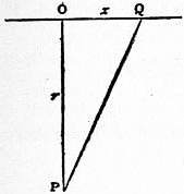
Fig. 1.

We will now consider in detail the important case in which uniform plane waves are resolved at a surface coincident with a wave-front (OQ). We imagine a wave-front divided into elementary rings or zones—often named after Huygens, but better after Fresnel—by spheres described round P (the point at which the aggregate effect is to be estimated), the first sphere, touching the plane at O, with a radius equal to PO, and the succeeding spheres with radii increasing at each step by ½λ. There are thus marked out a series of circles, whose radii x are given by x² + r² = (r + ½nλ)², or x² = nλr nearly; so that the rings are at first of nearly equal area. Now the effect upon P of each element of the plane is proportional to its area; but it depends also upon the distance from P, and possibly upon the inclination of the secondary ray to the direction of vibration and to the wave-front.

The latter question can only be treated in connexion with the dynamical theory (see below, § 11); but under all ordinary circumstances the result is independent of the precise answer that may be given. All that it is necessary to assume is that the effects of the successive zones gradually diminish, whether from the increasing obliquity of the secondary ray or because (on account of the limitation of the region of integration) the zones become at last more and more incomplete. The component vibrations at P due to the successive zones are thus nearly equal in amplitude and opposite in phase (the phase of each corresponding to that of the infinitesimal circle midway between the boundaries), and the series which we have to sum is one in which the terms are alternately opposite in sign and, while at first nearly constant in numerical magnitude, gradually diminish to zero. In such a series each term may be regarded as very nearly indeed destroyed by the halves of its immediate neighbours, and thus the sum of the whole series is represented by half the first term, which stands over uncompensated. The question is thus reduced to that of finding the effect of the first zone, or central circle, of which the area is πλr.

We have seen that the problem before us is independent of the law of the secondary wave as regards obliquity; but the result of the integration necessarily involves the law of the intensity and phase of a secondary wave as a function of r, the distance from the origin. And we may in fact, as was done by A. Smith (Camb. Math. Journ., 1843, 3, p. 46), determine the law of the secondary wave, by comparing the result of the integration with that obtained by supposing the primary wave to pass on to P without resolution.

Now as to the phase of the secondary wave, it might appear natural to suppose that it starts from any point Q with the phase of the primary wave, so that on arrival at P, it is retarded by the amount corresponding to QP. But a little consideration will prove that in that case the series of secondary waves could not reconstitute the primary wave. For the aggregate effect of the secondary waves is the half of that of the first Fresnel zone, and it is the central element only of that zone for which the distance to be travelled is equal to r. Let us conceive the zone in question to be divided into infinitesimal rings of equal area. The effects due to each of these rings are equal in amplitude and of phase ranging uniformly over half a complete period. The phase of the resultant is midway between those of the extreme elements, that is to say, a quarter of a period behind that due to the element at the centre of the circle. It is accordingly necessary to suppose that the secondary waves start with a phase one-quarter of a period in advance of that of the primary wave at the surface of resolution.

Further, it is evident that account must be taken of the variation of phase in estimating the magnitude of the effect at P of the first zone. The middle element alone contributes without deduction; the effect of every other must be found by introduction of a resolving factor, equal to cos θ, if θ represent the difference of phase between this element and the resultant. Accordingly, the amplitude of the resultant will be less than if all its components had the same phase, in the ratio

∫ +½π cos θdθ : π,

-½π

or 2 : π. Now 2 area /π = 2λr; so that, in order to reconcile the amplitude of the primary wave (taken as unity) with the half effect of the first zone, the amplitude, at distance r, of the secondary wave emitted from the element of area dS must be taken to be

dS/λr (1).

By this expression, in conjunction with the quarter-period acceleration of phase, the law of the secondary wave is determined.

That the amplitude of the secondary wave should vary as r-1 was to be expected from considerations respecting energy; but the occurrence of the factor λ-1, and the acceleration of phase, have sometimes been regarded as mysterious. It may be well therefore to remember that precisely these laws apply to a secondary wave of sound, which can be investigated upon the strictest mechanical principles.

The recomposition of the secondary waves may also be treated analytically. If the primary wave at O be cos kat, the effect of the secondary wave proceeding from the element dS at Q is

dS cos k(at − ρ + ¼λ) = − dS sin k(at − ρ).

λρ λρ

If dS = 2πxdx, we have for the whole effect

− 2π ∫ ∞ sin k(at − ρ)x dx ,

λ 0 ρ

or, since xdx = ρdρ, k = 2π/λ,

−k ∫ ∞ sin k(at − ρ)dρ = [ −cos k(at − ρ) ] ∞ .

r r

In order to obtain the effect of the primary wave, as retarded by traversing the distance r, viz. cos k(at − r), it is necessary to suppose that the integrated term vanishes at the upper limit. And it is important to notice that without some further understanding the integral is really ambiguous. According to the assumed law of the secondary wave, the result must actually depend upon the precise radius of the outer boundary of the region of integration, supposed to be exactly circular. This case is, however, at most very special and exceptional. We may usually suppose that a large number of the outer rings are incomplete, so that the integrated term at the upper limit may properly be taken to vanish. If a formal proof be desired, it may be obtained by introducing into the integral a factor such as e-hρ, in which h is ultimately made to diminish without limit.

When the primary wave is plane, the area of the first Fresnel zone is πλr, and, since the secondary waves vary as r-1, the intensity is independent of r, as of course it should be. If, however, the primary wave be spherical, and of radius a at the wave-front of resolution, then we know that at a distance r further on the amplitude of the primary wave will be diminished in the ratio a : (r + a). This may be regarded as a consequence of the altered area of the first Fresnel zone. For, if x be its radius, we have

{(r + ½λ)² − x²} + √ {a² − x²} = r + a,

so that

x² = λar/(a + r) nearly.

Since the distance to be travelled by the secondary waves is still r, we see how the effect of the first zone, and therefore of the whole series is proportional to a/(a + r). In like manner may be treated other cases, such as that of a primary wave-front of unequal principal curvatures.

The general explanation of the formation of shadows may also be conveniently based upon Fresnel’s zones. If the point under consideration be so far away from the geometrical shadow that a large number of the earlier zones are complete, then the illumination, determined sensibly by the first zone, is the same as if there were no obstruction at all. If, on the other hand, the point be well immersed in the geometrical shadow, the earlier zones are altogether missing, and, instead of a series of terms beginning with finite numerical magnitude and gradually diminishing to zero, we have now to deal with one of which the terms diminish to zero at both ends. The sum of such a series is very approximately zero, each term being neutralized by the halves of its immediate neighbours, which are of the opposite sign. The question of light or darkness then depends upon whether the series begins or ends abruptly. With few exceptions, abruptness can occur only in the presence of the first term, viz. when the secondary wave of least retardation is unobstructed, or when a ray passes through the point under consideration. According to the undulatory theory the light cannot be regarded strictly as travelling along a ray; but the existence of an unobstructed ray implies that the system of Fresnel’s zones can be commenced, and, if a large number of these zones are fully developed and do not terminate abruptly, the illumination is unaffected by the neighbourhood of obstacles. Intermediate cases in which a few zones only are formed belong especially to the province of diffraction.

An interesting exception to the general rule that full brightness requires the existence of the first zone occurs when the obstacle assumes the form of a small circular disk parallel to the plane of the incident waves. In the earlier half of the 18th century R. Delisle found that the centre of the circular shadow was occupied by a bright point of light, but the observation passed into oblivion until S. D. Poisson brought forward as an objection to Fresnel’s theory that it required at the centre of a circular shadow a point as bright as if no obstacle were intervening. If we conceive the primary wave to be broken up at the plane of the disk, a system of Fresnel’s zones can be constructed which begin from the circumference; and the first zone external to the disk plays the part ordinarily taken by the centre of the entire system. The whole effect is the half of that of the first existing zone, and this is sensibly the same as if there were no obstruction.

When light passes through a small circular or annular aperture, the illumination at any point along the axis depends upon the precise relation between the aperture and the distance from it at which the point is taken. If, as in the last paragraph, we imagine a system of zones to be drawn commencing from the inner circular boundary of the aperture, the question turns upon the manner in which the series terminates at the outer boundary. If the aperture be such as to fit exactly an integral number of zones, the aggregate effect may be regarded as the half of those due to the first and last zones. If the number of zones be even, the action of the first and last zones are antagonistic, and there is complete darkness at the point. If on the other hand the number of zones be odd, the effects conspire; and the illumination (proportional to the square of the amplitude) is four times as great as if there were no obstruction at all.

The process of augmenting the resultant illumination at a particular point by stopping some of the secondary rays may be carried much further (Soret, Pogg. Ann., 1875, 156, p. 99). By the aid of photography it is easy to prepare a plate, transparent where the zones of odd order fall, and opaque where those of even order fall. Such a plate has the power of a condensing lens, and gives an illumination out of all proportion to what could be obtained without it. An even greater effect (fourfold) can be attained by providing that the stoppage of the light from the alternate zones is replaced by a phase-reversal without loss of amplitude. R. W. Wood (Phil. Mag., 1898, 45, p 513) has succeeded in constructing zone plates upon this principle.

In such experiments the narrowness of the zones renders necessary a pretty close approximation to the geometrical conditions. Thus in the case of the circular disk, equidistant (r) from the source of light and from the screen upon which the shadow is observed, the width of the first exterior zone is given by

dx = λ(2r)/4(2x),

2x being the diameter of the disk. If 2r = 1000 cm., 2x = 1 cm., λ = 6 × 10-5 cm., then dx = .0015 cm. Hence, in order that this zone may be perfectly formed, there should be no error in the circumference of the order of .001 cm. (It is easy to see that the radius of the bright spot is of the same order of magnitude.) The experiment succeeds in a dark room of the length above mentioned, with a threepenny bit (supported by three threads) as obstacle, the origin of light being a small needle hole in a plate of tin, through which the sun’s rays shine horizontally after reflection from an external mirror. In the absence of a heliostat it is more convenient to obtain a point of light with the aid of a lens of short focus.

The amplitude of the light at any point in the axis, when plane waves are incident perpendicularly upon an annular aperture, is, as above,

cos k(at − r1) − cos k(at − r2) = 2 sin kat sin k(r1 − r2),

r2, r1 being the distances of the outer and inner boundaries from the point in question. It is scarcely necessary to remark that in all such cases the calculation applies in the first instance to homogeneous light, and that, in accordance with Fourier’s theorem, each homogeneous component of a mixture may be treated separately. When the original light is white, the presence of some components and the absence of others will usually give rise to coloured effects, variable with the precise circumstances of the case.

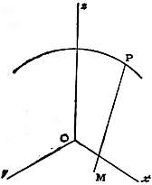
Fig. 2.

Although the matter can be fully treated only upon the basis of a dynamical theory, it is proper to point out at once that there is an element of assumption in the application of Huygens’s principle to the calculation of the effects produced by opaque screens of limited extent. Properly applied, the principle could not fail; but, as may readily be proved in the case of sonorous waves, it is not in strictness sufficient to assume the expression for a secondary wave suitable when the primary wave is undisturbed, with mere limitation of the integration to the transparent parts of the screen. But, except perhaps in the case of very fine gratings, it is probable that the error thus caused is insignificant; for the incorrect estimation of the secondary waves will be limited to distances of a few wave-lengths only from the boundary of opaque and transparent parts.

3. Fraunhofer’s Diffraction Phenomena.—A very general problem in diffraction is the investigation of the distribution of light over a screen upon which impinge divergent or convergent spherical waves after passage through various diffracting apertures. When the waves are convergent and the recipient screen is placed so as to contain the centre of convergency—the image of the original radiant point, the calculation assumes a less complicated form. This class of phenomena was investigated by J. von Fraunhofer (upon principles laid down by Fresnel), and are sometimes called after his name. We may conveniently commence with them on account of their simplicity and great importance in respect to the theory of optical instruments.

If ƒ be the radius of the spherical wave at the place of resolution, where the vibration is represented by cos kat, then at any point M (fig. 2) in the recipient screen the vibration due to an element dS of the wave-front is (§ 2)

− dS sin k(at − ρ),

λρ

ρ being the distance between M and the element dS.

Taking co-ordinates in the plane of the screen with the centre of the wave as origin, let us represent M by ξ, η, and P (where dS is situated) by x, y, z.

Then

ρ² = (x − ξ)² + (y − η)² + z², ƒ² = x² + y² + z²;

so that

ρ² = ƒ² − 2xξ − 2yη + ξ² + η².

In the applications with which we are concerned, ξ, η are very small quantities; and we may take

ρ = ƒ{ 1 − xξ + yη }.

ƒ²

At the same time dS may be identified with dxdy, and in the denominator ρ may be treated as constant and equal to ƒ. Thus the expression for the vibration at M becomes

− 1 ∫∫sin k { at − ƒ + xξ + yη } dxdy (1);

λƒ ƒ

and for the intensity, represented by the square of the amplitude,

I² = 1 [ ∫∫ sin k xξ + yη dxdy ] ²

벃² ƒ

+ 1 [ ∫∫ cos k xξ + yη dxdy ] ² (2).

벃² ƒ

This expression for the intensity becomes rigorously applicable when ƒ is indefinitely great, so that ordinary optical aberration disappears. The incident waves are thus plane, and are limited to a plane aperture coincident with a wave-front. The integrals are then properly functions of the direction in which the light is to be estimated.

In experiment under ordinary circumstances it makes no difference whether the collecting lens is in front of or behind the diffracting aperture. It is usually most convenient to employ a telescope focused upon the radiant point, and to place the diffracting apertures immediately in front of the object-glass. What is seen through the eye-piece in any case is the same as would be depicted upon a screen in the focal plane.

Before proceeding to special cases it may be well to call attention to some general properties of the solution expressed by (2) (see Bridge, Phil. Mag., 1858).

If when the aperture is given, the wave-length (proportional to k-1) varies, the composition of the integrals is unaltered, provided ξ and η are taken universely proportional to λ. A diminution of λ thus leads to a simple proportional shrinkage of the diffraction pattern, attended by an augmentation of brilliancy in proportion to λ-2.

If the wave-length remains unchanged, similar effects are produced by an increase in the scale of the aperture. The linear dimension of the diffraction pattern is inversely as that of the aperture, and the brightness at corresponding points is as the square of the area of aperture.

If the aperture and wave-length increase in the same proportion, the size and shape of the diffraction pattern undergo no change.

We will now apply the integrals (2) to the case of a rectangular aperture of width a parallel to x and of width b parallel to y. The limits of integration for x may thus be taken to be −½a and +½a, and for y to be −½b, +½b. We readily find (with substitution for k of 2π/λ)

· sin² πaξ · sin² πbη (3),

I² = a²b² ƒλ ƒλ

ƒ²λ² π²a²ξ² π²b²η²

ƒ²λ² ƒ²λ²

as representing the distribution of light in the image of a mathematical point when the aperture is rectangular, as is often the case in spectroscopes.

The second and third factors of (3) being each of the form sin²u/u², we have to examine the character of this function. It vanishes when u = mπ, m being any whole number other than zero. When u = 0, it takes the value unity. The maxima occur when

u = tan u, (4),

and then

sin²u / u² = cos²u (5).

To calculate the roots of (5) we may assume

u = (m + ½)π − y = U − y,

where y is a positive quantity which is small when u is large. Substituting this, we find cot y = U − y, whence

y = 1 (1 + y + y- + ...) − y³ − 2y5 − 17y7 .

U U U² 3 15 315

This equation is to be solved by successive approximation. It will readily be found that

u = U − y = U − U−1 − 2 U−3 − 13 U−5 − 146 U−7 − ... (6).

3 15 105

In the first quadrant there is no root after zero, since tan u > u, and in the second quadrant there is none because the signs of u and tan u are opposite. The first root after zero is thus in the third quadrant, corresponding to m = 1. Even in this case the series converges sufficiently to give the value of the root with considerable accuracy, while for higher values of m it is all that could be desired. The actual values of u/π (calculated in another manner by F. M. Schwerd) are 1.4303, 2.4590, 3.4709, 4.4747, 5.4818, 6.4844, &c.

Since the maxima occur when u = (m + ½)π nearly, the successive values are not very different from

4 , 4 , 4 , &c.

9π² 25π 49π²

The application of these results to (3) shows that the field is brightest at the centre ξ = 0, η = 0, viz. at the geometrical image of the radiant point. It is traversed by dark lines whose equations are

ξ = mfλ / a, η = mfλ / b.

Within the rectangle formed by pairs of consecutive dark lines, and not far from its centre, the brightness rises to a maximum; but these subsequent maxima are in all cases much inferior to the brightness at the centre of the entire pattern (ξ = 0, η = 0).

By the principle of energy the illumination over the entire focal plane must be equal to that over the diffracting area; and thus, in accordance with the suppositions by which (3) was obtained, its value when integrated from ξ = ∞ to ξ = +∞, and from η = −∞ to η = +∞ should be equal to ab. This integration, employed originally by P. Kelland (Edin. Trans. 15, p. 315) to determine the absolute intensity of a secondary wave, may be at once effected by means of the known formula

∫ +∞ sin²u du = ∫ +∞ sin u du = π.

−∞ u² −∞ u

It will be observed that, while the total intensity is proportional to ab, the intensity at the focal point is proportional to a²b². If the aperture be increased, not only is the total brightness over the focal plane increased with it, but there is also a concentration of the diffraction pattern. The form of (3) shows immediately that, if a and b be altered, the co-ordinates of any characteristic point in the pattern vary as a−1 and b−1.

The contraction of the diffraction pattern with increase of aperture is of fundamental importance in connexion with the resolving power of optical instruments. According to common optics, where images are absolute, the diffraction pattern is supposed to be infinitely small, and two radiant points, however near together, form separated images. This is tantamount to an assumption that λ is infinitely small. The actual finiteness of λ imposes a limit upon the separating or resolving power of an optical instrument.

This indefiniteness of images is sometimes said to be due to diffraction by the edge of the aperture, and proposals have even been made for curing it by causing the transition between the interrupted and transmitted parts of the primary wave to be less abrupt. Such a view of the matter is altogether misleading. What requires explanation is not the imperfection of actual images so much as the possibility of their being as good as we find them.

At the focal point (ξ = 0, η = 0) all the secondary waves agree in phase, and the intensity is easily expressed, whatever be the form of the aperture. From the general formula (2), if A be the area of aperture,

I0² = A² / 벃² (7).

The formation of a sharp image of the radiant point requires that the illumination become insignificant when ξ, η attain small values, and this insignificance can only arise as a consequence of discrepancies of phase among the secondary waves from various parts of the aperture. So long as there is no sensible discrepancy of phase there can be no sensible diminution of brightness as compared with that to be found at the focal point itself. We may go further, and lay it down that there can be no considerable loss of brightness until the difference of phase of the waves proceeding from the nearest and farthest parts of the aperture amounts to ¼λ.

When the difference of phase amounts to λ, we may expect the resultant illumination to be very much reduced. In the particular case of a rectangular aperture the course of things can be readily followed, especially if we conceive ƒ to be infinite. In the direction (suppose horizontal) for which η = 0, ξ/ƒ = sin θ, the phases of the secondary waves range over a complete period when sin θ = λ/a, and, since all parts of the horizontal aperture are equally effective, there is in this direction a complete compensation and consequent absence of illumination. When sin θ = 3⁄2λ/a, the phases range one and a half periods, and there is revival of illumination. We may compare the brightness with that in the direction θ = 0. The phase of the resultant amplitude is the same as that due to the central secondary wave, and the discrepancies of phase among the components reduce the amplitude in the proportion

1 ∫ +3⁄2π cos φ dφ: 1

3π −3⁄2π

or -2⁄3π : 1; so that the brightness in this direction is 4⁄9π² of the maximum at θ = 0. In like manner we may find the illumination in any other direction, and it is obvious that it vanishes when sin θ is any multiple of λ/a.

The reason of the augmentation of resolving power with aperture will now be evident. The larger the aperture the smaller are the angles through which it is necessary to deviate from the principal direction in order to bring in specified discrepancies of phase—the more concentrated is the image.