Part 1 — TABLE II

No. Elt. 1₁ 2₁ 2₂ 3₁ 3₂ 3₃ 4₁ 4₂ 4₃ 4₄ 5₁ 5₂ 5₃ 5₄ 5₅ 6₁ 6₂ 6₃ 6₄ 6₅ 6₆ 7₁ 7₂

1 H 1

2 He 2

3 Li 2 1

4 Be 2 2

5 B 2 2 (1)

6 C 2 2 2

7 N 2 4 1

8 O 2 4 2

9 F 2 4 3

10 Ne 2 4 4

11 Na 2 4 4 1

12 Mg 2 4 4 2

13 Al 2 4 4 2 1

14 Si 2 4 4 (2) (2)

15 P 2 4 4 4 1

16 S 2 4 4 4 2

17 Cl 2 4 4 4 3

18 A 2 4 4 4 4

19 K 2 4 4 4 4 - 1

20 Ca 2 4 4 4 4 - 2

21 Sc 2 4 4 4 4 1 (2)

22 Ti 2 4 4 4 4 2 (2)

29 Cu 2 4 4 6 6 6 1

30 Zn 2 4 4 6 6 6 2

31 Ga 2 4 4 6 6 6 2 1

32 Ge 2 4 4 6 6 6 4

33 As 2 4 4 6 6 6 4 1

34 Se 2 4 4 6 6 6 4 2

36 Kr 2 4 4 6 6 6 4 3

37 Rb 2 4 4 6 6 6 4 4 - - 1

38 Sr 2 4 4 6 6 6 4 4 - - 2

39 Y 2 4 4 6 6 6 4 4 1 - (2)

40 Zr 2 4 4 6 6 6 4 4 2 - (2)

47 Ag 2 4 4 6 6 6 6 6 6 - 1

48 Cd 2 4 4 6 6 6 6 6 6 - 2

49 In 2 4 4 6 6 6 6 6 6 - 2 1

50 Sn 2 4 4 6 6 6 6 6 6 - 4

51 Sb 2 4 4 6 6 6 6 6 6 - 4 1

52 Te 2 4 4 6 6 6 6 6 6 - 4 2

53 I 2 4 4 6 6 6 6 6 6 - 4 3

54 Xe 2 4 4 6 6 6 6 6 6 - 4 4

55 Cs 2 4 4 6 6 6 6 6 6 - 4 4 - - - 1

56 Ba 2 4 4 6 6 6 6 6 6 - 4 4 - - - 2

57 La 2 4 4 6 6 6 6 6 6 - 4 4 1 - - (2)

58 Ce 2 4 4 6 6 6 6 6 6 - 4 4 2 - - (2)

59 Pr 2 4 4 6 6 6 6 6 6 2 4 4 3 - - 1

71 Lu 2 4 4 6 6 6 8 8 8 8 4 4 1 - - (2)

72 Hf 2 4 4 6 6 6 8 8 8 8 4 4 2 - - (2)

79 Au 2 4 4 6 6 6 8 8 8 8 6 6 6 - - 1

80 Hg 2 4 4 6 6 6 8 8 8 8 6 6 6 - - 2

81 Ti 2 4 4 6 6 6 8 8 8 8 6 6 6 - - 2 1

82 Pb 2 4 4 6 6 6 8 8 8 8 6 6 6 - - (4)

83 Bi 2 4 4 6 6 6 8 8 8 8 6 6 6 - - 4 1

86 Rd 2 4 4 6 6 6 8 8 8 8 6 6 6 - - 4 4

88 Ra 2 4 4 6 6 6 8 8 8 8 6 6 6 - - 4 4 - - - - 2

89 Ac 2 4 4 6 6 6 8 8 8 8 6 6 6 - - 4 4 1 - - - (2)

90 Th 2 4 4 6 6 6 8 8 8 8 6 6 6 - - 4 4 2 - - - (2)

118 ? 2 4 4 6 6 6 8 8 8 8 8 8 8 8 - 6 6 6 - - - 4 4

The table also gives the number of spectroscopic valency electrons, a quantity which is required by the theory of thermal ionization. The spectroscopic valency electrons are those in equivalent outer orbits (outer orbits of equal total quantum number which have the same azimuthal quantum number). The number is not necessarily the same as the number of chemical valencies (the number of orbits with the same total quantum number) although the two values coincide for the alkali metals and for the alkaline earths. For carbon,[6] on the other hand, the number of spectroscopic valency electrons is two (the number of 22 orbits), while the chemical valency, corresponding to the total number of 2-quantum orbits, is four.

THE PRODUCTION OF LINE SPECTRA

It is not proposed to discuss the theory of the origin of line spectra here in any detail. What is important from the astrophysical point of view is the association of known lines in the spectrum with different levels of energy in the atom, these levels representing definite electron orbits. Absorption and emission of energy take place in an atom by the transfer of an electron from an orbit associated with low energy to an orbit associated with high energy, and vice versa. The frequency of the light which is thus absorbed or emitted is expressed by the familiar quantum relation:

where and are the initial and final energies, , and is the frequency of the light absorbed or given out.

The atom absorbs from its environment the quanta relevant to the particular electron transfers of which it is capable at the time. These transfers are, of course, governed by the number and arrangement of the spectroscopic valency electrons, or in other words, by the state of ionization or excitation of the atom.

The unionized (or neutral) atom in the unexcited state absorbs the ultimate lines by the removal of one electron from its normal stationary state to some other which can be reached from that state, and re-emits them by the return of the electron to that state. The electron may, of course, leave the state to which it was carried by the ultimate absorption and pass to some state other than the normal one. If this final state is a state of higher energy than the previous state, the line produced by the process will be an absorption line; if it is of lower energy the result will be the production of an emission line. In either case the line produced by the transfer of an electron from a stationary state other than the normal state is known as a subordinate line. The distinction between series of ultimate and subordinate lines is of great importance in the astrophysical applications of the theory of ionization.

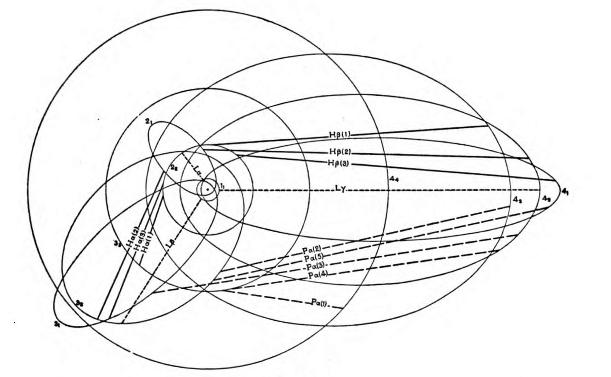
Figure 2

The hydrogen atom. The ten innermost orbits possible for the single electron of the atom of hydrogen are diagrammatically represented. All possible quantum transitions between the orbits are indicated as follows:—short dashes, Lyman series, terminating at a 1-quantum orbit; full lines, Balmer series, terminating at a 2-quantum orbit; long dashes, Paschen series, terminating at a 3-quantum orbit. Transfers are only possible between orbits with azimuthal quantum numbers differing by ±1.

When the energy supply from the environment is great enough, the “outermost” (or most easily detachable) valency electron is entirely removed by the energy absorbed. In consequence the atom is superficially transformed, giving rise to a totally new spectrum, which strongly resembles the spectrum of the atom next preceding in the periodic system. Bohr’s table embodies the interpretation of this resemblance—the so-called Displacement Rule of Kossell and Sommerfeld[7]—which has recently been strikingly confirmed by a very complete investigation of the arc and spark (neutral and ionized) spectra of the atoms in the first long period.[8] It may be seen at once, for instance, that the removal of the outermost (or ) electron from the atom of aluminum () produces an arrangement of external electrons identical with that for magnesium (). The ionized atom produced by the complete removal of one electron gives, like the neutral atom, two kinds of line spectrum—the ultimate lines and the subordinate lines.

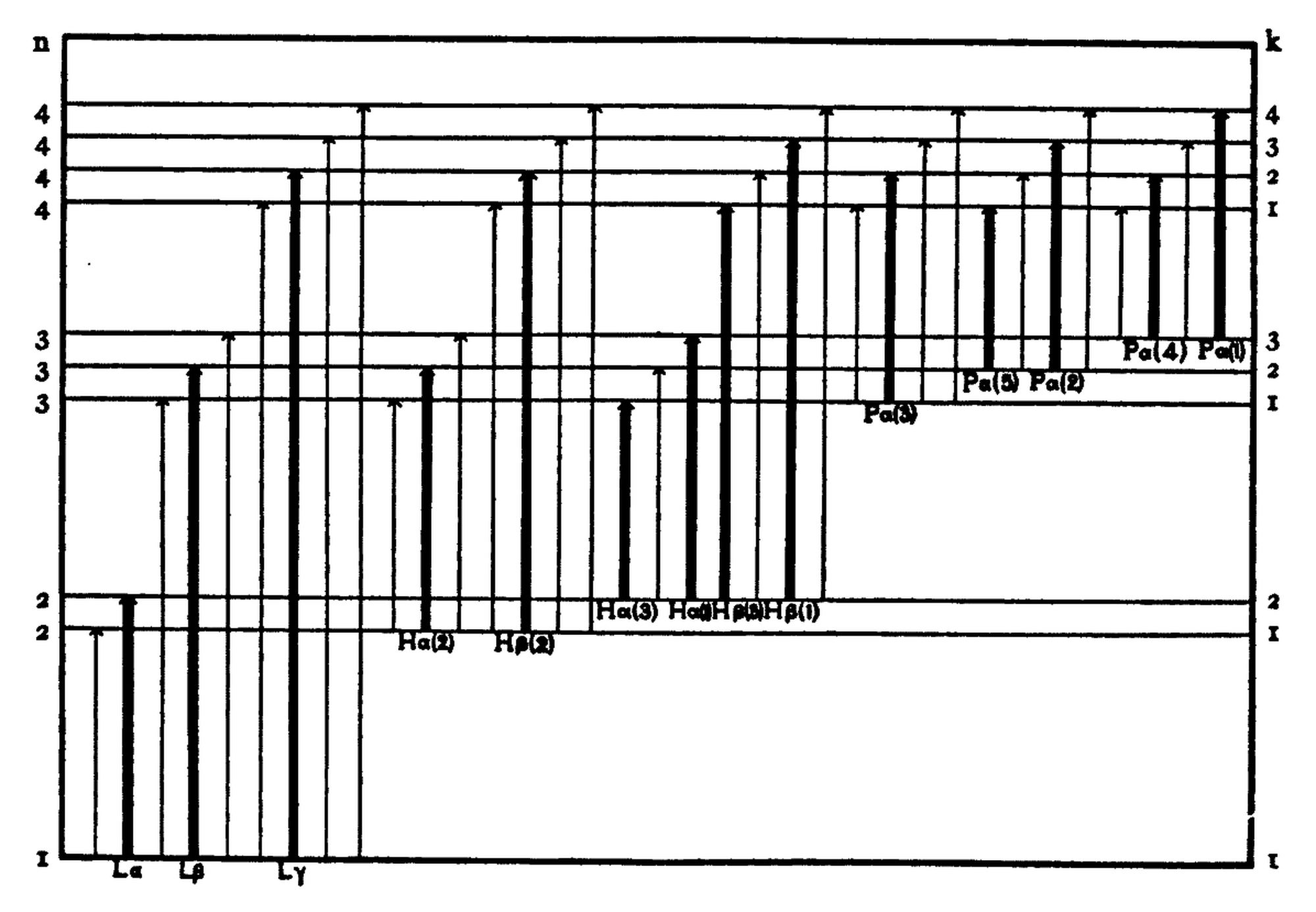
Figure 3

Energy levels for the hydrogen atom. Horizontal lines represent diagrammatically the levels of energy corresponding to all the possible electron orbits up to and including those of total quantum number four. Total quantum numbers are indicated on the left margin, azimuthal quantum numbers on the right margin. Transitions are only possible between orbits which differ by ±1 in azimuthal quantum number. All such possible transitions are indicated in the diagram by heavy lines. “Forbidden jumps,” for which the difference in azimuthal quantum number is zero or greater than 1, are indicated by light lines. This diagram embodies the same relations as Figure 2, the levels representing the various orbits in that figure.

Effectively, the ionized atom may be regarded as a new atom altogether. It reproduces the spectrum of the atom of preceding atomic number, in cases which have been fully investigated, with great fidelity, excepting that the Rydberg constant in the series formula is multiplied by four. For the twice and thrice ionized atoms the same is true, the Rydberg constant being multiplied by nine and by sixteen in the two cases. It is scarcely necessary to mention the beautiful confirmation of the theory that has been furnished by the analyses[9][10] of the spectra of Na, Mg, and Mg+, Al, Al+, and Al++, and Si, Si+, Si++, and Si+++. The attribution of the Pickering series (first observed in the spectrum of Puppis) to ionized helium was the first established example of the displacement rule, and constituted one of the earliest triumphs of the Bohr theory.[11] The detection and resolution of the alternate components of that series, which fall very near to the Balmer lines of hydrogen in the spectra of the hottest stars, and the consequent derivation of the Rydberg constant for helium,[12] represents an astrophysical contribution to pure physics which is of the highest importance.

IONIZATION AND EXCITATION

The ionization potential of an atom is the energy in volts that is required in order to remove the outermost electron to infinity. The excitation potential corresponding to any particular spectral series is the energy in volts that must be imparted to the atom in the normal state in order that there may be an electron in a suitable electron orbit for the absorption or emission of that series. Several different excitation potentials are usually associated with one atom. The ionization potential and the excitation potentials are collectively termed the critical potentials.

From the astrophysical point of view, ionization and excitation potentials are important as forming the basic data for the Saha theory of thermal ionization, with which the greater part of this work is concerned. A list of the ionization potentials hitherto determined is therefore reproduced in the following table. The first two columns contain the values obtained by the physical and spectroscopic methods, respectively. The third column contains “astrophysical estimates,” which are inserted here to make the table more complete. The derivation of the astrophysical values will be discussed[13] in Chapter XI. Physical values result from the direct application of electrical potentials to the element in question, and spectroscopic values are derived from the values of the optical terms. (See Appendix.)