VOLUME XIV SLICE I Husband to Hydrolysis (continued 8)

The time taken by the float in passing over the measured distance may be observed by a chronograph, started as the float passes the upper rope or line, and stopped when it passes the lower. In Cunningham’s observations two chronometers were sometimes used, the time of passing one end of the run being noted on one, and that of passing the other end of the run being noted on the other. The chronometers were compared immediately before the observations. In other cases a single chronometer was used placed midway of the run. The moment of the floats passing the ends of the run was signalled to a time-keeper at the chronometer by shouting. It was found quite possible to count the chronometer beats to the nearest half second, and in some cases to the nearest quarter second.

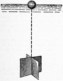
Fig. 137.

§ 137. Sub-surface Floats.—The velocity at different depths below the surface of a stream may be obtained by sub-surface floats, used precisely in the same way as surface floats. The most usual arrangement is to have a large float, of slightly greater density than water, connected with a small and very light surface float. The motion of the combined arrangement is not sensibly different from that of the large float, and the small surface float enables an observer to note the path and velocity of the sub-surface float. The instrument is, however, not free from objection. If the large submerged float is made of very nearly the same density as water, then it is liable to be thrown upwards by very slight eddies in the water, and it does not maintain its position at the depth at which it is intended to float. On the other hand, if the large float is made sensibly heavier than water, the indicating or surface float must be made rather large, and then it to some extent influences the motion of the submerged float. Fig. 137 shows one form of sub-surface float. It consists of a couple of tin plates bent at a right angle and soldered together at the angle. This is connected with a wooden ball at the surface by a very thin wire or cord. As the tin alone makes a heavy submerged float, it is better to attach to the tin float some pieces of wood to diminish its weight in water. Fig. 138 shows the form of submerged float used by Cunningham. It consists of a hollow metal ball connected to a slice of cork, which serves as the surface float.

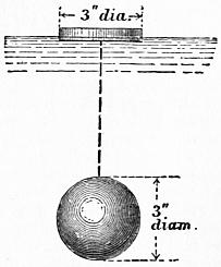
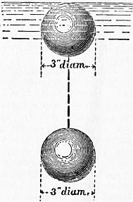
Fig. 138. Fig. 139.

§ 138. Twin Floats.—Suppose two equal and similar floats (fig. 139) connected by a wire. Let one float be a little lighter and the other a little heavier than water. Then the velocity of the combined floats will be the mean of the surface velocity and the velocity at the depth at which the heavier float swims, which is determined by the length of the connecting wire. Thus if vs is the surface velocity and vd the velocity at the depth to which the lower float is sunk, the velocity of the combined floats will be

v = 1⁄2 (vs + vd).

Consequently, if v is observed, and vs determined by an experiment with a single float,

vd = 2v − vs

According to Cunningham, the twin float gives better results than the sub-surface float.

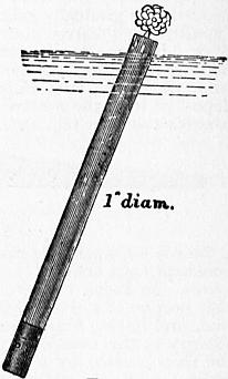
Fig. 140.

§ 139. Velocity Rods.—Another form of float is shown in fig. 140. This consists of a cylindrical rod loaded at the lower end so as to float nearly vertical in water. A wooden rod, with a metal cap at the bottom in which shot can be placed, answers better than anything else, and sometimes the wooden rod is made in lengths, which can be screwed together so as to suit streams of different depths. A tuft of cotton wool at the top serves to make the float more easily visible. Such a rod, so adjusted in length that it sinks nearly to the bed of the stream, gives directly the mean velocity of the whole vertical section in which it floats.

§ 140. Revy’s Current Meter.—No instrument has been so much used in directly determining the velocity of a stream at a given point as the screw current meter. Of this there are a dozen varieties at least. As an example of the instrument in its simplest form, Revy’s meter may be selected. This is an ordinary screw meter of a larger size than usual, more carefully made, and with its details carefully studied (figs. 141, 142). It was designed after experience in gauging the great South American rivers. The screw, which is actuated by the water, is 6 in. in diameter, and is of the type of the Griffiths screw used in ships. The hollow spherical boss serves to make the weight of the screw sensibly equal to its displacement, so that friction is much reduced. On the axis aa of the screw is a worm which drives the counter. This consists of two worm wheels g and h fixed on a common axis. The worm wheels are carried on a frame attached to the pin l. By means of a string attached to l they can be pulled into gear with the worm, or dropped out of gear and stopped at any instant. A nut m can be screwed up, if necessary, to keep the counter permanently in gear. The worm is two-threaded, and the worm wheel g has 200 teeth. Consequently it makes one rotation for 100 rotations of the screw, and the number of rotations up to 100 is marked by the passage of the graduations on its edge in front of a fixed index. The second worm wheel has 196 teeth, and its edge is divided into 49 divisions. Hence it falls behind the first wheel one division for a complete rotation of the latter. The number of hundreds of rotations of the screw are therefore shown by the number of divisions on h passed over by an index fixed to g. One difficulty in the use of the ordinary screw meter is that particles of grit, getting into the working parts, very sensibly alter the friction, and therefore the speed of the meter. Revy obviates this by enclosing the counter in a brass box with a glass face. This box is filled with pure water, which ensures a constant coefficient of friction for the rubbing parts, and prevents any mud or grit finding its way in. In order that the meter may place itself with the axis parallel to the current, it is pivoted on a vertical axis and directed by a large vane shown in fig. 142. To give the vane more directing power the vertical axis is nearer the screw than in ordinary meters, and the vane is larger. A second horizontal vane is attached by the screws x, x, the object of which is to allow the meter to rest on the ground without the motion of the screw being interfered with. The string or wire for starting and stopping the meter is carried through the centre of the vertical axis, so that the strain on it may not tend to pull the meter oblique to the current. The pitch of the screw is about 9 in. The screws at x serve for filling the meter with water. The whole apparatus is fixed to a rod (fig. 142), of a length proportionate to the depth, or for very great depths it is fixed to a weighted bar lowered by ropes, a plan invented by Revy. The instrument is generally used thus. The reading of the counter is noted, and it is put out of gear. The meter is then lowered into the water to the required position from a platform between two boats, or better from a temporary bridge. Then the counter is put into gear for one, two or five minutes. Lastly, the instrument is raised and the counter again read. The velocity is deduced from the number of rotations in unit time by the formulae given below. For surface velocities the counter may be kept permanently in gear, the screw being started and stopped by hand.

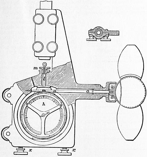
Fig. 141.

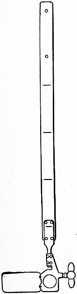
Fig. 142.

§ 141. The Harlacher Current Meter.—In this the ordinary counting apparatus is abandoned. A worm drives a worm wheel, which makes an electrical contact once for each 100 rotations of the worm. This contact gives a signal above water. With this arrangement, a series of velocity observations can be made, without removing the instrument from the water, and a number of practical difficulties attending the accurate starting and stopping of the ordinary counter are entirely got rid of. Fig. 143 shows the meter. The worm wheel z makes one rotation for 100 of the screw. A pin moving the lever x makes the electrical contact. The wires b, c are led through a gas pipe B; this also serves to adjust the meter to any required position on the wooden rod dd. The rudder or vane is shown at WH. The galvanic current acts on the electromagnet m, which is fixed in a small metal box containing also the battery. The magnet exposes and withdraws a coloured disk at an opening in the cover of the box.

§ 142. Amsler Laffon Current Meter.—A very convenient and accurate current meter is constructed by Amsler Laffon of Schaffhausen. This can be used on a rod, and put into and out of gear by a ratchet. The peculiarity in this case is that there is a double ratchet, so that one pull on the string puts the counter into gear and a second puts it out of gear. The string may be slack during the action of the meter, and there is less uncertainty than when the counter has to be held in gear. For deep streams the meter A is suspended by a wire with a heavy lenticular weight below (fig. 144). The wire is payed out from a small winch D, with an index showing the depth of the meter, and passes over a pulley B. The meter is in gimbals and is directed by a conical rudder which keeps it facing the stream with its axis horizontal. There is an electric circuit from a battery C through the meter, and a contact is made closing the circuit every 100 revolutions. The moment the circuit closes a bell rings. By a subsidiary arrangement, when the foot of the instrument, 0.3 metres below the axis of the meter, touches the ground the circuit is also closed and the bell rings. It is easy to distinguish the continuous ring when the ground is reached from the short ring when the counter signals. A convenient winch for the wire is so graduated that if set when the axis of the meter is at the water surface it indicates at any moment the depth of the meter below the surface. Fig. 144 shows the meter as used on a boat. It is a very convenient instrument for obtaining the velocity at different depths and can also be used as a sounding instrument.

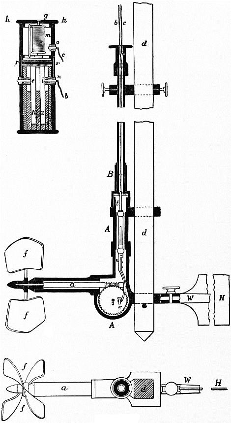
Fig. 143.

§ 143. Determination of the Coefficients of the Current Meter.—Suppose a series of observations has been made by towing the meter in still water at different speeds, and that it is required to ascertain from these the constants of the meter. If v is the velocity of the water and n the observed number of rotations per second, let

v = α + βn

(1)

where α and β are constants. Now let the meter be towed over a measured distance L, and let N be the revolutions of the meter and t the time of transit. Then the speed of the meter relatively to the water is L/t = v feet per second, and the number of revolutions per second is N/t = n. Suppose m observations have been made in this way, furnishing corresponding values of v and n, the speed in each trial being as uniform as possible,

Σn = n1 + n2 + ...

Σv = v1 + v2 + ...

Σnv = n1v1 + n2v2 + ...

Σn2 = n12 + n22 + ...

[Σn]2 = [n1 + n2 + ...]2

Then for the determination of the constants α and β in (1), by the method of least squares—

α = Σn2Σv − ΣnΣnv ,

mΣn2 − [Σn]2

β = mΣnv − ΣvΣn .

mΣn2 − [Σn]2

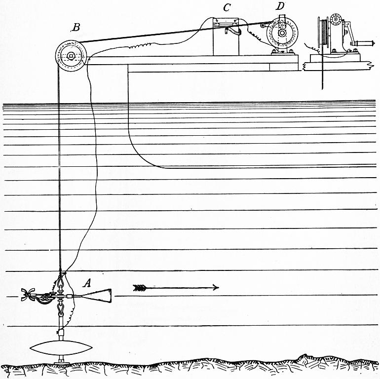
Fig. 144.

In a few cases the constants for screw current meters have been determined by towing them in R. E. Froude’s experimental tank in which the resistance of ship models is ascertained. In that case the data are found with exceptional accuracy.

§ 144. Darcy Gauge or modified Pitot Tube.—A very old instrument for measuring velocities, invented by Henri Pitot in 1730 (Histoire de l’Académie des Sciences, 1732, p. 376), consisted simply of a vertical glass tube with a right-angled bend, placed so that its mouth was normal to the direction of flow (fig. 145).

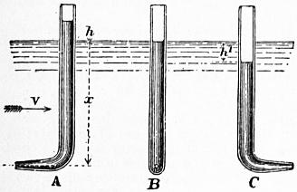
Fig. 145.

The impact of the stream on the mouth of the tube balances a column in the tube, the height of which is approximately h = v2/2g, where v is the velocity at the depth x. Placed with its mouth parallel to the stream the water inside the tube is nearly at the same level as the surface of the stream, and turned with the mouth down stream, the fluid sinks a depth h′ = v2/2g nearly, though the tube in that case interferes with the free flow of the liquid and somewhat modifies the result. Pitot expanded the mouth of the tube so as to form a funnel or bell mouth. In that case he found by experiment

h = 1.5v2 / 2g.

But there is more disturbance of the stream. Darcy preferred to make the mouth of the tube very small to avoid interference with the stream and to check oscillations of the water column. Let the difference of level of a pair of tubes A and B (fig. 145) be taken to be h = kv2/2g, then k may be taken to be a corrective coefficient whose value in well-shaped instruments is very nearly unity. By placing his instrument in front of a boat towed through water Darcy found k = 1.034; by placing the instrument in a stream the velocity of which had been ascertained by floats, he found k = 1.006; by readings taken in different parts of the section of a canal in which a known volume of water was flowing, he found k = 0.993. He believed the first value to be too high in consequence of the disturbance caused by the boat. The mean of the other two values is almost exactly unity (Recherches hydrauliques, Darcy and Bazin, 1865, p. 63). W. B. Gregory used somewhat differently formed Pitot tubes for which the k = 1 (Am. Soc. Mech. Eng., 1903, 25). T. E. Stanton used a Pitot tube in determining the velocity of an air current, and for his instrument he found k = 1.030 to k = 1.032 (“On the Resistance of Plane Surfaces in a Current of Air,” Proc. Inst. Civ. Eng., 1904, 156).

One objection to the Pitot tube in its original form was the great difficulty and inconvenience of reading the height h in the immediate neighbourhood of the stream surface. This is obviated in the Darcy gauge, which can be removed from the stream to be read.

Fig. 146 shows a Darcy gauge. It consists of two Pitot tubes having their mouths at right angles. In the instrument shown, the two tubes, formed of copper in the lower part, are united into one for strength, and the mouths of the tubes open vertically and horizontally. The upper part of the tubes is of glass, and they are provided with a brass scale and two verniers b, b. The whole instrument is supported on a vertical rod or small pile AA, the fixing at B permitting the instrument to be adjusted to any height on the rod, and at the same time allowing free rotation, so that it can be held parallel to the current. At c is a two-way cock, which can be opened or closed by cords. If this is shut, the instrument can be lifted out of the stream for reading. The glass tubes are connected at top by a brass fixing, with a stop cock a, and a flexible tube and mouthpiece m. The use of this is as follows. If the velocity is required at a point near the surface of the stream, one at least of the water columns would be below the level at which it could be read. It would be in the copper part of the instrument. Suppose then a little air is sucked out by the tube m, and the cock a closed, the two columns will be forced up an amount corresponding to the difference between atmospheric pressure and that in the tubes. But the difference of level will remain unaltered.

When the velocities to be measured are not very small, this instrument is an admirable one. It requires observation only of a single linear quantity, and does not require any time observation. The law connecting the velocity and the observed height is a rational one, and it is not absolutely necessary to make any experiments on the coefficient of the instrument. If we take v = k√(2gh), then it appears from Darcy’s experiments that for a well-formed instrument k does not sensibly differ from unity. It gives the velocity at a definite point in the stream. The chief difficulty arises from the fact that at any given point in a stream the velocity is not absolutely constant, but varies a little from moment to moment. Darcy in some of his experiments took several readings, and deduced the velocity from the mean of the highest and lowest.

§ 145. Perrodil Hydrodynamometer.—This consists of a frame abcd (fig. 147) placed vertically in the stream, and of a height not less than the stream’s depth. The two vertical members of this frame are connected by cross bars, and united above water by a circular bar, situated in the vertical plane and carrying a horizontal graduated circle ef. This whole system is movable round its axis, being suspended on a pivot at g connected with the fixed support mn. Other horizontal arms serve as guides. The central vertical rod gr forms a torsion rod, being fixed at r to the frame abcd, and, passing freely upwards through the guides, it carries a horizontal needle moving over the graduated circle ef. The support g, which carries the apparatus, also receives in a tubular guide the end of the torsion rod gr and a set screw for fixing the upper end of the torsion rod when necessary. The impulse of the stream of water is received on a circular disk x, in the plane of the torsion rod and the frame abcd. To raise and lower the apparatus easily, it is not fixed directly to the rod mn, but to a tube kl sliding on mn.

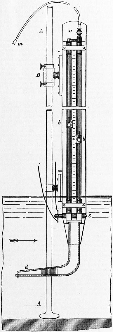
Fig. 146.

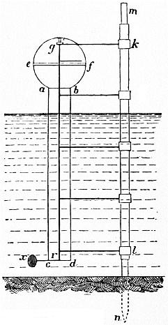
Fig. 147.

Suppose the apparatus arranged so that the disk x is at that level in the stream where the velocity is to be determined. The plane abcd is placed parallel to the direction of motion of the water. Then the disk x (acting as a rudder) will place itself parallel to the stream on the down stream side of the frame. The torsion rod will be unstrained, and the needle will be at zero on the graduated circle. If, then, the instrument is turned by pressing the needle, till the plane abcd of the disk and the zero of the graduated circle is at right angles to the stream, the torsion rod will be twisted through an angle which measures the normal impulse of the stream on the disk x. That angle will be given by the distance of the needle from zero. Observation shows that the velocity of the water at a given point is not constant. It varies between limits more or less wide. When the apparatus is nearly in its right position, the set screw at g is made to clamp the torsion spring. Then the needle is fixed, and the apparatus carrying the graduated circle oscillates. It is not, then, difficult to note the mean angle marked by the needle.

Let r be the radius of the torsion rod, l its length from the needle over ef to r, and α the observed torsion angle. Then the moment of the couple due to the molecular forces in the torsion rod is

M = EtIα / l;

where Et is the modulus of elasticity for torsion, and I the polar moment of inertia of the section of the rod. If the rod is of circular section, I = 1⁄2πr4. Let R be the radius of the disk, and b its leverage, or the distance of its centre from the axis of the torsion rod. The moment of the pressure of the water on the disk is

Fb = kb (G / 2g) πR2v2,

where G is the heaviness of water and k an experimental coefficient. Then

EtIα / l = kb (G / 2g) πR2v2.

For any given instrument,

v = c √ α,

where c is a constant coefficient for the instrument.

The instrument as constructed had three disks which could be used at will. Their radii and leverages were in feet

R = b =

1st disk 0.052 0.16

2nd ” 0.105 0.32

3rd ” 0.210 0.66

For a thin circular plate, the coefficient k = 1.12. In the actual instrument the torsion rod was a brass wire 0.06 in. diameter and 61⁄2 ft. long. Supposing α measured in degrees, we get by calculation

v = 0.335 √ α; 0.115 √ α; 0.042 √ α.

Very careful experiments were made with the instrument. It was fixed to a wooden turning bridge, revolving over a circular channel of 2 ft. width, and about 76 ft. circumferential length. An allowance was made for the slight current produced in the channel. These experiments gave for the coefficient c, in the formula v = c√α,

1st disk, c = 0.3126 for velocities of 3 to 16 ft. 2nd disk, c = 0.1177 for velocities of 11⁄4 to 31⁄4 ft. 3rd disk, c = 0.0349 for velocities of less than 11⁄4 ft.

The instrument is preferable to the current meter in giving the velocity in terms of a single observed quantity, the angle of torsion, while the current meter involves the observation of two quantities, the number of rotations and the time. The current meter, except in some improved forms, must be withdrawn from the water to read the result of each experiment, and the law connecting the velocity and number of rotations of a current meter is less well-determined than that connecting the pressure on a disk and the torsion of the wire of a hydrodynamometer.

The Pitot tube, like the hydrodynamometer, does not require a time observation. But, where the velocity is a varying one, and consequently the columns of water in the Pitot tube are oscillating, there is room for doubt as to whether, at any given moment of closing the cock, the difference of level exactly measures the impulse of the stream at the moment. The Pitot tube also fails to give measurable indications of very low velocities.

Processes for Gauging Streams

§ 146. Gauging by Observation of the Maximum Surface Velocity.—The method of gauging which involves the least trouble is to determine the surface velocity at the thread of the stream, and to deduce from it the mean velocity of the whole cross section. The maximum surface velocity may be determined by floats or by a current meter. Unfortunately the ratio of the maximum surface to the mean velocity is extremely variable. Thus putting v0 for the surface velocity at the thread of the stream, and vm for the mean velocity of the whole cross section, vm/v0 has been found to have the following values:—

vm/v0

De Prony, experiments on small wooden channels 0.8164

Experiments on the Seine 0.62

Destrem and De Prony, experiments on the Neva 0.78

Boileau, experiments on canals 0.82

Baumgartner, experiments on the Garonne 0.80

Brünings (mean) 0.85

Cunningham, Solani aqueduct 0.823

Various formulae, either empirical or based on some theory of the vertical and horizontal velocity curves, have been proposed for determining the ratio vm/v0. Bazin found from his experiments the empirical expression

vm = v0 − 25.4 √ (mi);

where m is the hydraulic mean depth and i the slope of the stream.

In the case of irrigation canals and rivers, it is often important to determine the discharge either daily or at other intervals of time, while the depth and consequently the mean velocity is varying. Cunningham (Roorkee Prof. Papers, iv. 47), has shown that, for a given part of such a stream, where the bed is regular and of permanent section, a simple formula may be found for the variation of the central surface velocity with the depth. When once the constants of this formula have been determined by measuring the central surface velocity and depth, in different conditions of the stream, the surface velocity can be obtained by simply observing the depth of the stream, and from this the mean velocity and discharge can be calculated. Let z be the depth of the stream, and v0 the surface velocity, both measured at the thread of the stream. Then v02 = cz; where c is a constant which for the Solani aqueduct had the values 1.9 to 2, the depths being 6 to 10 ft., and the velocities 31⁄2 to 41⁄2 ft. Without any assumption of a formula, however, the surface velocities, or still better the mean velocities, for different conditions of the stream may be plotted on a diagram in which the abscissae are depths and the ordinates velocities. The continuous curve through points so found would then always give the velocity for any observed depth of the stream, without the need of making any new float or current meter observations.

§ 147. Mean Velocity determined by observing a Series of Surface Velocities.—The ratio of the mean velocity to the surface velocity in one longitudinal section is better ascertained than the ratio of the central surface velocity to the mean velocity of the whole cross section. Suppose the river divided into a number of compartments by equidistant longitudinal planes, and the surface velocity observed in each compartment. From this the mean velocity in each compartment and the discharge can be calculated. The sum of the partial discharges will be the total discharge of the stream. When wires or ropes can be stretched across the stream, the compartments can be marked out by tags attached to them. Suppose two such ropes stretched across the stream, and floats dropped in above the upper rope. By observing within which compartment the path of the float lies, and noting the time of transit between the ropes, the surface velocity in each compartment can be ascertained. The mean velocity in each compartment is 0.85 to 0.91 of the surface velocity in that compartment. Putting k for this ratio, and v1, v2 ... for the observed velocities, in compartments of area Ω1, Ω2 ... then the total discharge is

Q = k (Ω1v1 + Ω2v2 + ... ).

If several floats are allowed to pass over each compartment, the mean of all those corresponding to one compartment is to be taken as the surface velocity of that compartment.

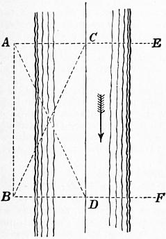
Fig. 148.

This method is very applicable in the case of large streams or rivers too wide to stretch a rope across. The paths of the floats are then ascertained in this way. Let fig. 148 represent a portion of the river, which should be straight and free from obstructions. Suppose a base line AB measured parallel to the thread of the stream, and let the mean cross section of the stream be ascertained either by sounding the terminal cross sections AE, BF, or by sounding a series of equidistant cross sections. The cross sections are taken at right angles to the base line. Observers are placed at A and B with theodolites or box sextants. The floats are dropped in from a boat above AE, and picked up by another boat below BF. An observer with a chronograph or watch notes the time in which each float passes from AE to BF. The method of proceeding is this. The observer A sets his theodolite in the direction AE, and gives a signal to drop a float. B keeps his instrument on the float as it comes down. At the moment the float arrives at C in the line AE, the observer at A calls out. B clamps his instrument and reads off the angle ABC, and the time observer begins to note the time of transit. B now points his instrument in the direction BF, and A keeps the float on the cross wire of his instrument. At the moment the float arrives at D in the line BF, the observer B calls out, A clamps his instrument and reads off the angle BAD, and the time observer notes the time of transit from C to D. Thus all the data are determined for plotting the path CD of the float and determining its velocity. By dropping in a series of floats, a number of surface velocities can be determined. When all these have been plotted, the river can be divided into convenient compartments. The observations belonging to each compartment are then averaged, and the mean velocity and discharge calculated. It is obvious that, as the surface velocity is greatly altered by wind, experiments of this kind should be made in very calm weather.

The ratio of the surface velocity to the mean velocity in the same vertical can be ascertained from the formulae for the vertical velocity curve already given (§ 101). Exner, in Erbkam’s Zeitschrift for 1875, gave the following convenient formula. Let v be the mean and V the surface velocity in any given vertical longitudinal section, the depth of which is h

v / V = (1 + 0.1478 √ h) / (1 + 0.2216 √ h).

If vertical velocity rods are used instead of common floats, the mean velocity is directly determined for the vertical section in which the rod floats. No formula of reduction is then necessary. The observed velocity has simply to be multiplied by the area of the compartment to which it belongs.

§ 148. Mean Velocity of the Stream from a Series of Mid Depth Velocities.—In the gaugings of the Mississippi it was found that the mid depth velocity differed by only a very small quantity from the mean velocity in the vertical section, and it was uninfluenced by wind. If therefore a series of mid depth velocities are determined by double floats or by a current meter, they may be taken to be the mean velocities of the compartments in which they occur, and no formula of reduction is necessary. If floats are used, the method is precisely the same as that described in the last paragraph for surface floats. The paths of the double floats are observed and plotted, and the mean taken of those corresponding to each of the compartments into which the river is divided. The discharge is the sum of the products of the observed mean mid depth velocities and the areas of the compartments.

§ 149. P. P. Boileau’s Process for Gauging Streams.—Let U be the mean velocity at a given section of a stream, V the maximum velocity, or that of the principal filament, which is generally a little below the surface, W and w the greatest and least velocities at the surface. The distance of the principal filament from the surface is generally less than one-fourth of the depth of the stream; W is a little less than V; and U lies between W and w. As the surface velocities change continuously from the centre towards the sides there are at the surface two filaments having a velocity equal to U. The determination of the position of these filaments, which Boileau terms the gauging filaments, cannot be effected entirely by theory. But, for sections of a stream in which there are no abrupt changes of depth, their position can be very approximately assigned. Let Δ and l be the horizontal distances of the surface filament, having the velocity W, from the gauging filament, which has the velocity U, and from the bank on one side. Then

Δ / l = c4 √ {(W + 2w) / 7 (W − w)},

c being a numerical constant. From gaugings by Humphreys and Abbot, Bazin and Baumgarten, the values c = 0.919, 0.922 and 0.925 are obtained. Boileau adopts as a mean value 0.922. Hence, if W and w are determined by float gauging or otherwise, Δ can be found, and then a single velocity observation at Δ ft. from the filament of maximum velocity gives, without need of any reduction, the mean velocity of the stream. More conveniently W, w, and U can be measured from a horizontal surface velocity curve, obtained from a series of float observations.

§ 150. Direct Determination of the Mean Velocity by a Current Meter or Darcy Gauge.—The only method of determining the mean velocity at a cross section of a stream which involves no assumption of the ratio of the mean velocity to other quantities is this—a plank bridge is fixed across the stream near its surface. From this, velocities are observed at a sufficient number of points in the cross section of the stream, evenly distributed over its area. The mean of these is the true mean velocity of the stream. In Darcy and Bazin’s experiments on small streams, the velocity was thus observed at 36 points in the cross section.

When the stream is too large to fix a bridge across it, the observations may be taken from a boat, or from a couple of boats with a gangway between them, anchored successively at a series of points across the width of the stream. The position of the boat for each series of observations is fixed by angular observations to a base line on shore.

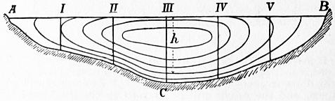
Fig. 149.

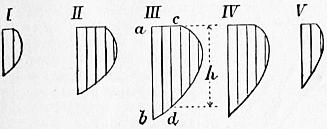
Fig. 150.

§ 151. A. R. Harlacher’s Graphic Method of determining the Discharge from a Series of Current Meter Observations.—Let ABC (fig. 149) be the cross section of a river at which a complete series of current meter observations have been taken. Let I., II., III., ... be the verticals at different points of which the velocities were measured. Suppose the depths at I., II., III., ... (fig. 149), set off as vertical ordinates in fig. 150, and on these vertical ordinates suppose the velocities set off horizontally at their proper depths. Thus, if v is the measured velocity at the depth h from the surface in fig. 149, on vertical marked III., then at III. in fig. 150 take cd = h and ac = v. Then d is a point in the vertical velocity curve for the vertical III., and, all the velocities for that ordinate being similarly set off, the curve can be drawn. Suppose all the vertical velocity curves I.... V. (fig. 150), thus drawn. On each of these figures draw verticals corresponding to velocities of x, 2x, 3x ... ft. per second. Then for instance cd at III. (fig. 150) is the depth at which a velocity of 2x ft. per second existed on the vertical III. in fig. 149 and if cd is set off at III. in fig. 149 it gives a point in a curve passing through points of the section where the velocity was 2x ft. per second. Set off on each of the verticals in fig. 149 all the depths thus found in the corresponding diagram in fig. 150. Curves drawn through the corresponding points on the verticals are curves of equal velocity.

The discharge of the stream per second may be regarded as a solid having the cross section of the river (fig. 149) as a base, and cross sections normal to the plane of fig. 149 given by the diagrams in fig. 150. The curves of equal velocity may therefore be considered as contour lines of the solid whose volume is the discharge of the stream per second. Let Ω0 be the area of the cross section of the river, Ω1, Ω2 ... the areas contained by the successive curves of equal velocity, or, if these cut the surface of the stream, by the curves and that surface. Let x be the difference of velocity for which the successive curves are drawn, assumed above for simplicity at 1 ft. per second. Then the volume of the successive layers of the solid body whose volume represents the discharge, limited by successive planes passing through the contour curves, will be

1⁄2 x (Ω0 + Ω1), 1⁄2 x (Ω1 + Ω2), and so on.

Consequently the discharge is

Q = x {1⁄2 (Ω0 + Ωn) + Ω1 = Ω2 + ... + Ωn−1}.

The areas Ω0, Ω1 ... are easily ascertained by means of the polar planimeter. A slight difficulty arises in the part of the solid lying above the last contour curve. This will have generally a height which is not exactly x, and a form more rounded than the other layers and less like a conical frustum. The volume of this may be estimated separately, and taken to be the area of its base (the area Ωn) multiplied by 1⁄3 to 1⁄2 its height.

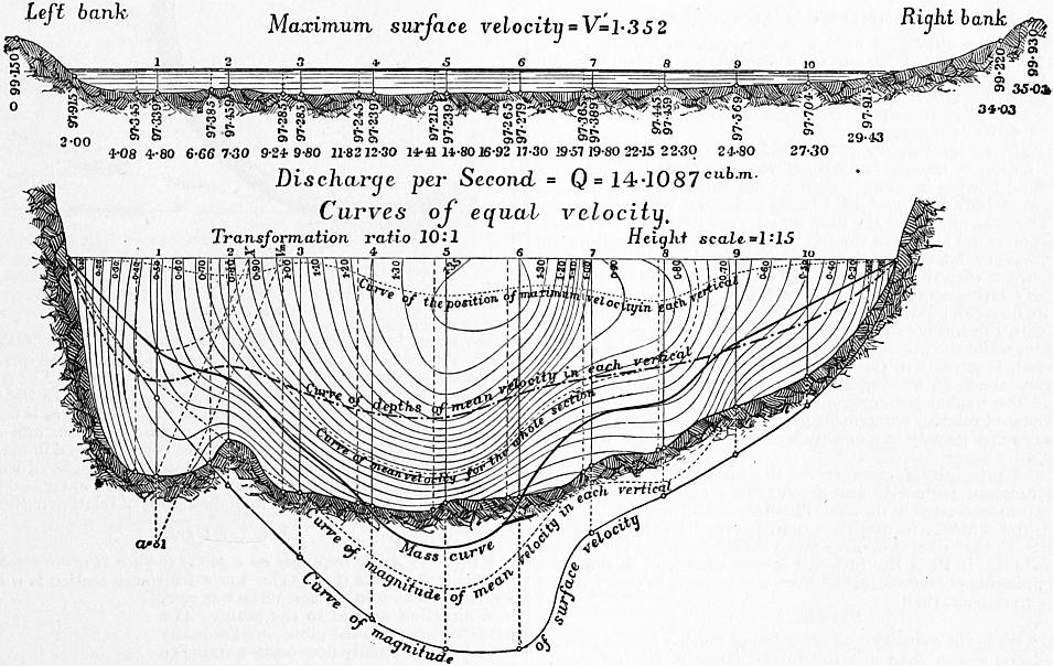
Fig. 151.

Fig. 151 shows the results of one of Harlacher’s gaugings worked out in this way. The upper figure shows the section of the river and the positions of the verticals at which the soundings and gaugings were taken. The lower gives the curves of equal velocity, worked out from the current meter observations, by the aid of vertical velocity curves. The vertical scale in this figure is ten times as great as in the other. The discharge calculated from the contour curves is 14.1087 cubic metres per second. In the lower figure some other interesting curves are drawn. Thus, the uppermost dotted curve is the curve through points at which the maximum velocity was found; it shows that the maximum velocity was always a little below the surface, and at a greater depth at the centre than at the sides. The next curve shows the depth at which the mean velocity for each vertical was found. The next is the curve of equal velocity corresponding to the mean velocity of the stream; that is, it passes through points in the cross section where the velocity was identical with the mean velocity of the stream.

Hydraulic Machines

§ 152. Hydraulic machines may be broadly divided into two classes: (1) Motors, in which water descending from a higher to a lower level, or from a higher to a lower pressure, gives up energy which is available for mechanical operations; (2) Pumps, in which the energy of a steam engine or other motor is expended in raising water from a lower to a higher level. A few machines such as the ram and jet pump combine the functions of motor and pump. It may be noted that constructively pumps are essentially reversed motors. The reciprocating pump is a reversed pressure engine, and the centrifugal pump a reversed turbine. Hydraulic machine tools are in principle motors combined with tools, and they now form an important special class.

Water under pressure conveyed in pipes is a convenient and economical means of transmitting energy and distributing it to many scattered working points. Hence large and important hydraulic systems are adopted in which at a central station water is pumped at high pressure into distributing mains, which convey it to various points where it actuates hydraulic motors operating cranes, lifts, dock gates, and in some cases riveting and shearing machines. In this case the head driving the hydraulic machinery is artificially created, and it is the convenience of distributing power in an easily applied form to distant points which makes the system advantageous. As there is some unavoidable loss in creating an artificial head this system is most suitable for driving machines which work intermittently (see Power Transmission). The development of electrical methods of transmitting and distributing energy has led to the utilization of many natural waterfalls so situated as to be useless without such a means of transferring the power to points where it can be conveniently applied. In some cases, as at Niagara, the hydraulic power can only be economically developed in very large units, and it can be most conveniently subdivided and distributed by transformation into electrical energy. Partly from the development of new industries such as paper-making from wood pulp and electro-metallurgical processes, which require large amounts of cheap power, partly from the facility with which energy can now be transmitted to great distances electrically, there has been a great increase in the utilization of water-power in countries having natural waterfalls. According to the twelfth census of the United States the total amount of water-power reported as used in manufacturing establishments in that country was 1,130,431 h.p. in 1870; 1,263,343 h.p. in 1890; and 1,727,258 h.p. in 1900. The increase was 8.4% in the decade 1870-1880, 3.1% in 1880-1890, and no less than 36.7% in 1890-1900. The increase is the more striking because in this census the large amounts of hydraulic power which are transmitted electrically are not included.

XII. IMPACT AND REACTION OF WATER

§ 153. When a stream of fluid in steady motion impinges on a solid surface, it presses on the surface with a force equal and opposite to that by which the velocity and direction of motion of the fluid are changed. Generally, in problems on the impact of fluids, it is necessary to neglect the effect of friction between the fluid and the surface on which it moves.

During Impact the Velocity of the Fluid relatively to the Surface on which it impinges remains unchanged in Magnitude.—Consider a mass of fluid flowing in contact with a solid surface also in motion, the motion of both fluid and solid being estimated relatively to the earth. Then the motion of the fluid may be resolved into two parts, one a motion equal to that of the solid, and in the same direction, the other a motion relatively to the solid. The motion which the fluid has in common with the solid cannot at all be influenced by the contact. The relative component of the motion of the fluid can only be altered in direction, but not in magnitude. The fluid moving in contact with the surface can only have a relative motion parallel to the surface, while the pressure between the fluid and solid, if friction is neglected, is normal to the surface. The pressure therefore can only deviate the fluid, without altering the magnitude of the relative velocity. The unchanged common component and, combined with it, the deviated relative component give the resultant final velocity, which may differ greatly in magnitude and direction from the initial velocity.

From the principle of momentum, the impulse of any mass of fluid reaching the surface in any given time is equal to the change of momentum estimated in the same direction. The pressure between the fluid and surface, in any direction, is equal to the change of momentum in that direction of so much fluid as reaches the surface in one second. If Pa is the pressure in any direction, m the mass of fluid impinging per second, va the change of velocity in the direction of Pa due to impact, then

Pa = mva.

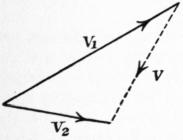
Fig. 152.

If v1 (fig. 152) is the velocity and direction of motion before impact, v2 that after impact, then v is the total change of motion due to impact. The resultant pressure of the fluid on the surface is in the direction of v, and is equal to v multiplied by the mass impinging per second. That is, putting P for the resultant pressure,

P = mv.

Let P be resolved into two components, N and T, normal and tangential to the direction of motion of the solid on which the fluid impinges. Then N is a lateral force producing a pressure on the supports of the solid, T is an effort which does work on the solid. If u is the velocity of the solid, Tu is the work done per second by the fluid in moving the solid surface.

Let Q be the volume, and GQ the weight of the fluid impinging per second, and let v1 be the initial velocity of the fluid before striking the surface. Then GQv12/2g is the original kinetic energy of Q cub. ft. of fluid, and the efficiency of the stream considered as an arrangement for moving the solid surface is

η = Tu / (GQv12 / 2g).

§ 154. Jet deviated entirely in one Direction.—Geometrical Solution (fig. 153).—Suppose a jet of water impinges on a surface ac with a velocity ab, and let it be wholly deviated in planes parallel to the figure. Also let ae be the velocity and direction of motion of the surface. Join eb; then the water moves with respect to the surface in the direction and with the velocity eb. As this relative velocity is unaltered by contact with the surface, take cd = eb, tangent to the surface at c, then cd is the relative motion of the water with respect to the surface at c. Take df equal and parallel to ae. Then fc (obtained by compounding the relative motion of water to surface and common velocity of water and surface) is the absolute velocity and direction of the water leaving the surface. Take ag equal and parallel to fc. Then, since ab is the initial and ag the final velocity and direction of motion, gb is the total change of motion of the water. The resultant pressure on the plane is in the direction gb. Join eg. In the triangle gae, ae is equal and parallel to df, and ag to fc. Hence eg is equal and parallel to cd. But cd = eb = relative motion of water and surface. Hence the change of motion of the water is represented in magnitude and direction by the third side of an isosceles triangle, of which the other sides are equal to the relative velocity of the water and surface, and parallel to the initial and final directions of relative motion.

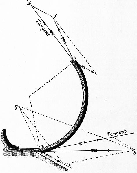
Fig. 153.

Special Cases

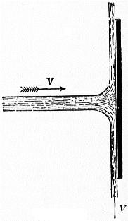
Fig. 154.

§ 155. (1) A Jet impinges on a plane surface at rest, in a direction normal to the plane (fig. 154).—Let a jet whose section is ω impinge with a velocity v on a plane surface at rest, in a direction normal to the plane. The particles approach the plane, are gradually deviated, and finally flow away parallel to the plane, having then no velocity in the original direction of the jet. The quantity of water impinging per second is ωv. The pressure on the plane, which is equal to the change of momentum per second, is P = (G/g) ωv2.

(2) If the plane is moving in the direction of the jet with the velocity ±u, the quantity impinging per second is ω(v ± u). The momentum of this quantity before impact is (G/g)ω(v ± u)v. After impact, the water still possesses the velocity ±u in the direction of the jet; and the momentum, in that direction, of so much water as impinges in one second, after impact, is ±(G/g) ω (v ± u)u. The pressure on the plane, which is the change of momentum per second, is the difference of these quantities or P = (G/g) ω (v ± u)2. This differs from the expression obtained in the previous case, in that the relative velocity of the water and plane v ± u is substituted for v. The expression may be written P = 2 × G × ω (v ± u)2/2g, where the last two terms are the volume of a prism of water whose section is the area of the jet and whose length is the head due to the relative velocity. The pressure on the plane is twice the weight of that prism of water. The work done when the plane is moving in the same direction as the jet is Pu = (G/g) ω (v − u)2u foot-pounds per second. There issue from the jet ωv cub. ft. per second, and the energy of this quantity before impact is (G/2g) ωv3. The efficiency of the jet is therefore η = 2(v − u)2u/v3. The value of u which makes this a maximum is found by differentiating and equating the differential coefficient to zero:—

dη / du = 2 (v2 − 4vu + 3u2) / v3 = 0;

∴ u = v or 1⁄3 v.

The former gives a minimum, the latter a maximum efficiency.

Putting u = 1⁄3v in the expression above,

η max. = 8⁄27.

(3) If, instead of one plane moving before the jet, a series of planes are introduced at short intervals at the same point, the quantity of water impinging on the series will be ωv instead of ω(v − u), and the whole pressure = (G/g) ωv (v − u). The work done is (G/g)ωvu (v − u). The efficiency η = (G/g) ωvu (v − u) ÷ (G/2g) ωv3 = 2u(v-u)/v2. This becomes a maximum for dη/du = 2(v − 2u) = 0, or u = 1⁄2v, and the η = 1⁄2. This result is often used as an approximate expression for the velocity of greatest efficiency when a jet of water strikes the floats of a water wheel. The work wasted in this case is half the whole energy of the jet when the floats run at the best speed.

§ 156. (4) Case of a Jet impinging on a Concave Cup Vane, velocity of water v, velocity of vane in the same direction u (fig. 155), weight impinging per second = Gw (v − u).

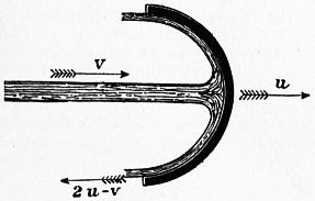
Fig. 155.

If the cup is hemispherical, the water leaves the cup in a direction parallel to the jet. Its relative velocity is v − u when approaching the cup, and −(v − u) when leaving it. Hence its absolute velocity when leaving the cup is u − (v − u) = 2u − v. The change of momentum per second = (G/g) ω (v − u) {v − (2u − v)} = 2(G/g) ω (v − u)2. Comparing this with case 2, it is seen that the pressure on a hemispherical cup is double that on a flat plane. The work done on the cup = 2(G/g) ω (v − u) 2u foot-pounds per second. The efficiency of the jet is greatest when v = 3u; in that case the efficiency = 16⁄27.

If a series of cup vanes are introduced in front of the jet, so that the quantity of water acted upon is ωv instead of ω(v − u), then the whole pressure on the chain of cups is (G/g) ωv {v − (2u − v)} = 2(G/g)ωv (v − u). In this case the efficiency is greatest when v = 2u, and the maximum efficiency is unity, or all the energy of the water is expended on the cups.

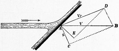
Fig. 156.

§ 157. (5) Case of a Flat Vane oblique to the Jet (fig. 156).—This case presents some difficulty. The water spreading on the plane in all directions from the point of impact, different particles leave the plane with different absolute velocities. Let AB = v = velocity of water, AC = u = velocity of plane. Then, completing the parallelogram, AD represents in magnitude and direction the relative velocity of water and plane. Draw AE normal to the plane and DE parallel to the plane. Then the relative velocity AD may be regarded as consisting of two components, one AE normal, the other DE parallel to the plane. On the assumption that friction is insensible, DE is unaffected by impact, but AE is destroyed. Hence AE represents the entire change of velocity due to impact and the direction of that change. The pressure on the plane is in the direction AE, and its amount is = mass of water impinging per second × AE.

Let DAE = θ, and let AD = vr. Then AE = vr cos θ; DE = vr sin θ. If Q is the volume of water impinging on the plane per second, the change of momentum is (G/g) Qvr cos θ. Let AC = u = velocity of the plane, and let AC make the angle CAE = δ with the normal to the plane. The velocity of the plane in the direction AE = u cos δ. The work of the jet on the plane = (G/g) Qvr cos θ u cos δ. The same problem may be thus treated algebraically (fig. 157). Let BAF = α, and CAF = δ. The velocity v of the water may be decomposed into AF = v cos α normal to the plane, and FB = v sin α parallel to the plane. Similarly the velocity of the plane = u = AC = BD can be decomposed into BG = FE = u cos δ normal to the plane, and DG = u sin δ parallel to the plane. As friction is neglected, the velocity of the water parallel to the plane is unaffected by the impact, but its component v cos α normal to the plane becomes after impact the same as that of the plane, that is, u cos δ. Hence the change of velocity during impact = AE = v cos α − u cos δ. The change of momentum per second, and consequently the normal pressure on the plane is N = (G/g) Q(v cos α − u cos δ). The pressure in the direction in which the plane is moving is P = N cos δ = (G/g)Q (v cos α − u cos δ) cos δ, and the work done on the plane is Pu = (G/g)Q(v cos α − u cos δ) u cos δ, which is the same expression as before, since AE = vr cos θ = v cos α − u cos δ.

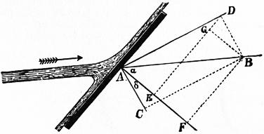
Fig. 157.

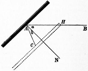
Fig. 158.

In one second the plane moves so that the point A (fig. 158) comes to C, or from the position shown in full lines to the position shown in dotted lines. If the plane remained stationary, a length AB = v of the jet would impinge on the plane, but, since the plane moves in the same direction as the jet, only the length HB = AB − AH impinges on the plane.

But AH = AC cos δ / cos α = u cos δ / cos α, and therefore HB = v − u cos δ / cos α. Let ω = sectional area of jet; volume impinging on plane per second = Q = ω(v − u cos δ / cos α) = ω (v cos α − u cos δ) / cos α. Inserting this in the formulae above, we get

N = G ω (v cos α − u cos δ)2;

g cos α

(1)

P = G ω cos δ (v cos α − u cos δ)2;

g cos α

(2)

Pu = G ωu cos δ (v cos α − u cos δ)2;

g cos α

(3)

Three cases may be distinguished:—

(a) The plane is at rest. Then u = 0, N = (G/g) ωv2cos α; and the work done on the plane and the efficiency of the jet are zero.

(b) The plane moves parallel to the jet. Then δ = α, and Pu = (G/g)ωu cos2 α (v − u)2, which is a maximum when u = 1⁄3v.

When u = 1⁄3v then Pu max. = 4⁄27(G/g)ωv3 cos2α, and the efficiency = η = 4⁄9cos2α.

(c) The plane moves perpendicularly to the jet. Then δ = 90° − α; cos δ = sin α; and Pu = G/g ωu (sin α / cos α) (v cos α − u sin α)2. This is a maximum when u = 1⁄3v cos α.

When u = 1⁄3v cos α, the maximum work and the efficiency are the same as in the last case.

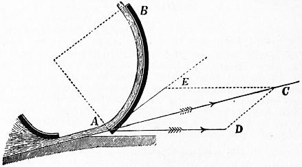
Fig. 159.

§ 158. Best Form of Vane to receive Water.—When water impinges normally or obliquely on a plane, it is scattered in all directions after impact, and the work carried away by the water is then generally lost, from the impossibility of dealing afterwards with streams of water deviated in so many directions. By suitably forming the vane, however, the water may be entirely deviated in one direction, and the loss of energy from agitation of the water is entirely avoided.

Let AB (fig. 159) be a vane, on which a jet of water impinges at the point A and in the direction AC. Take AC = v = velocity of water, and let AD represent in magnitude and direction the velocity of the vane. Completing the parallelogram, DC or AE represents the direction in which the water is moving relatively to the vane. If the lip of the vane at A is tangential to AE, the water will not have its direction suddenly changed when it impinges on the vane, and will therefore have no tendency to spread laterally. On the contrary it will be so gradually deviated that it will glide up the vane in the direction AB. This is sometimes expressed by saying that the vane receives the water without shock.

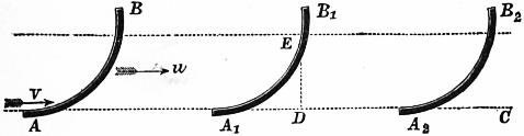
Fig. 160.

§ 159. Floats of Poncelet Water Wheels.—Let AC (fig. 160) represent the direction of a thin horizontal stream of water having the velocity v. Let AB be a curved float moving horizontally with velocity u. The relative motion of water and float is then initially horizontal, and equal to v − u.

In order that the float may receive the water without shock, it is necessary and sufficient that the lip of the float at A should be tangential to the direction AC of relative motion. At the end of (v − u)/g seconds the float moving with the velocity u comes to the position A1B1, and during this time a particle of water received at A and gliding up the float with the relative velocity v − u, attains a height DE = (v − u)2/2g. At E the water comes to relative rest. It then descends along the float, and when after 2(v − u)/g seconds the float has come to A2B2 the water will again have reached the lip at A2 and will quit it tangentially, that is, in the direction CA2, with a relative velocity −(v − u) = −√ (2gDE) acquired under the influence of gravity. The absolute velocity of the water leaving the float is therefore u − (v − u) = 2u − v. If u = 1⁄2v, the water will drop off the bucket deprived of all energy of motion. The whole of the work of the jet must therefore have been expended in driving the float. The water will have been received without shock and discharged without velocity. This is the principle of the Poncelet wheel, but in that case the floats move over an arc of a large circle; the stream of water has considerable thickness (about 8 in.); in order to get the water into and out of the wheel, it is then necessary that the lip of the float should make a small angle (about 15°) with the direction of its motion. The water quits the wheel with a little of its energy of motion remaining.

§ 160. Pressure on a Curved Surface when the Water is deviated wholly in one Direction.—When a jet of water impinges on a curved surface in such a direction that it is received without shock, the pressure on the surface is due to its gradual deviation from its first direction. On any portion of the area the pressure is equal and opposite to the force required to cause the deviation of so much water as rests on that surface. In common language, it is equal to the centrifugal force of that quantity of water.

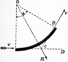
Fig. 161.

Case 1. Surface Cylindrical and Stationary.—Let AB (fig. 161) be the surface, having its axis at O and its radius = r. Let the water impinge at A tangentially, and quit the surface tangentially at B. Since the surface is at rest, v is both the absolute velocity of the water and the velocity relatively to the surface, and this remains unchanged during contact with the surface, because the deviating force is at each point perpendicular to the direction of motion. The water is deviated through an angle BCD = AOB = φ. Each particle of water of weight p exerts radially a centrifugal force pv2/rg. Let the thickness of the stream = t ft. Then the weight of water resting on unit of surface = Gt ℔; and the normal pressure per unit of surface = n = Gtv2/gr. The resultant of the radial pressures uniformly distributed from A to B will be a force acting in the direction OC bisecting AOB, and its magnitude will equal that of a force of intensity = n, acting on the projection of AB on a plane perpendicular to the direction OC. The length of the chord AB = 2r sin 1⁄2φ; let b = breadth of the surface perpendicular to the plane of the figure. The resultant pressure on surface

= R = 2rb sin φ × Gt · v2 = 2 G btv2 sin φ ,

2 g r g 2

which is independent of the radius of curvature. It may be inferred that the resultant pressure is the same for any curved surface of the same projected area, which deviates the water through the same angle.

Case 2. Cylindrical Surface moving in the Direction AC with Velocity u.—The relative velocity = v − u. The final velocity BF (fig. 162) is found by combining the relative velocity BD = v − u tangential to the surface with the velocity BE = u of the surface. The intensity of normal pressure, as in the last case, is (G/g) t (v − u)2/r. The resultant normal pressure R = 2(G/g) bt (v − u)2 sin 1⁄2φ. This resultant pressure may be resolved into two components P and L, one parallel and the other perpendicular to the direction of the vane’s motion. The former is an effort doing work on the vane. The latter is a lateral force which does no work.

P = R sin 1⁄2φ = (G/g) bt (v − u)2 (1 − cos φ); L = R cos 1⁄2φ = (G/g) bt (v − u)2 sin φ.

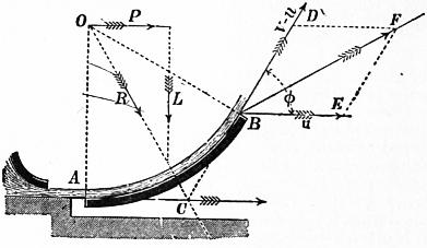
Fig. 162.

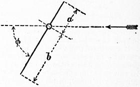
Fig. 163.

The work done by the jet on the vane is Pu = (G/g) btu (v − u)2(1 − cos φ), which is a maximum when u = 1⁄3v. This result can also be obtained by considering that the work done on the plane must be equal to the energy lost by the water, when friction is neglected.

If φ = 180°, cos φ = −1, 1 − cos φ = 2; then P = 2(G/g) bt (v − u)2, the same result as for a concave cup.

§ 161. Position which a Movable Plane takes in Flowing Water.—When a rectangular plane, movable about an axis parallel to one of its sides, is placed in an indefinite current of fluid, it takes a position such that the resultant of the normal pressures on the two sides of the axis passes through the axis. If, therefore, planes pivoted so that the ratio a/b (fig. 163) is varied are placed in water, and the angle they make with the direction of the stream is observed, the position of the resultant of the pressures on the plane is determined for different angular positions. Experiments of this kind have been made by Hagen. Some of his results are given in the following table:—

Larger plane. Smaller Plane.

a/b = 1.0 φ = ... φ = 90°

0.9 75° 721⁄2°

0.8 60° 57°

0.7 48° 43°

0.6 25° 29°

0.5 13° 13°

0.4 8° 61⁄2°

0.3 6° ..

0.2 4° ..

§ 162. Direct Action distinguished from Reaction (Rankine, Steam Engine, § 147).

The pressure which a jet exerts on a vane can be distinguished into two parts, viz∴—

(1) The pressure arising from changing the direct component of the velocity of the water into the velocity of the vane. In fig. 153, § 154, ab cos bae is the direct component of the water’s velocity, or component in the direction of motion of vane. This is changed into the velocity ae of the vane. The pressure due to direct impulse is then

P1 = GQ (ab cos bae − ae) / g.

For a flat vane moving normally, this direct action is the only action producing pressure on the vane.

(2) The term reaction is applied to the additional action due to the direction and velocity with which the water glances off the vane. It is this which is diminished by the friction between the water and the vane. In Case 2, § 160, the direct pressure is

P1 = Gbt (v − u)2 / g.

That due to reaction is

P2 = −Gbt (v − u)2 cos φ / g.

If φ < 90°, the direct component of the water’s motion is not wholly converted into the velocity of the vane, and the whole pressure due to direct impulse is not obtained. If φ > 90°, cos φ is negative and an additional pressure due to reaction is obtained.

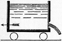
Fig. 164.

§ 163. Jet Propeller.—In the case of vessels propelled by a jet of water (fig. 164), driven sternwards from orifices at the side of the vessel, the water, originally at rest outside the vessel, is drawn into the ship and caused to move with the forward velocity V of the ship. Afterwards it is projected sternwards from the jets with a velocity v relatively to the ship, or v − V relatively to the earth. If Ω is the total sectional area of the jets, Ωv is the quantity of water discharged per second. The momentum generated per second in a sternward direction is (G/g) Ωv (v − V), and this is equal to the forward acting reaction P which propels the ship.

The energy carried away by the water

= 1⁄2 (G/g) Ωv (v − V)2.

(1)

The useful work done on the ship

PV = (G/g) Ωv (v − V) V.

(2)

Adding (1) and (2), we get the whole work expended on the water, neglecting friction:—

W = 1⁄2 (G/g) Ωv (v2 − V2).

Hence the efficiency of the jet propeller is

PV/W = 2V / (v + V).

(3)

This increases towards unity as v approaches V. In other words, the less the velocity of the jets exceeds that of the ship, and therefore the greater the area of the orifice of discharge, the greater is the efficiency of the propeller.

In the “Waterwitch” v was about twice V. Hence in this case the theoretical efficiency of the propeller, friction neglected, was about 2⁄3.

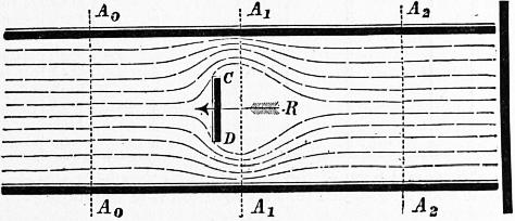
Fig. 165.

§ 164. Pressure of a Steady Stream in a Uniform Pipe on a Plane normal to the Direction of Motion.—Let CD (fig. 165) be a plane placed normally to the stream which, for simplicity, may be supposed to flow horizontally. The fluid filaments are deviated in front of the plane, form a contraction at A1A1, and converge again, leaving a mass of eddying water behind the plane. Suppose the section A0A0 taken at a point where the parallel motion has not begun to be disturbed, and A2A2 where the parallel motion is re-established. Then since the same quantity of water with the same velocity passes A0A0, A2A2 in any given time, the external forces produce no change of momentum on the mass A0A0A2A2, and must therefore be in equilibrium. If Ω is the section of the stream at A0A0 or A2A2, and ω the area of the plate CD, the area of the contracted section of the stream at A1A1 will be cc(Ω − ω), where cc is the coefficient of contraction. Hence, if v is the velocity at A0A0 or A2A2, and v1 the velocity at A1A1,

vΩ = ccv (Ω − ω);

∴ v1 = vΩ / cc (Ω − ω).

(1)

Let p0, p1, p2 be the pressures at the three sections. Applying Bernoulli’s theorem to the sections A0A0 and A1A1,

p0 + v2 = p1 + v12 .

G 2g G 2g

Also, for the sections A1A1 and A2A2, allowing that the head due to the relative velocity v1 − v is lost in shock:—

p1 + v12 = p2 + v2 + (v1 − v)2 ;

G 2g G 2g 2g

∴ p0 − p2 = G (v1 − v)2 / 2g;

(2)

or, introducing the value in (1),

p0 − p2 = G ( Ω − 1 ) 2 v2

2g cc (Ω − ω)

(3)

Now the external forces in the direction of motion acting on the mass A0A0A2A2 are the pressures p0Ω1 − p2Ω at the ends, and the reaction −R of the plane on the water, which is equal and opposite to the pressure of the water on the plane. As these are in equilibrium,

(p0 − p2) Ω − R = 0;

∴ R = GΩ ( Ω − 1 ) 2 v2 ;

cc (Ω − ω) 2g

(4)

an expression like that for the pressure of an isolated jet on an indefinitely extended plane, with the addition of the term in brackets, which depends only on the areas of the stream and the plane. For a given plane the expression in brackets diminishes as Ω increases. If Ω/ω = ρ, the equation (4) becomes

R = Gω v2 { ρ ( ρ − 1 ) 2 },

2g cc (ρ − 1)

(4a)

which is of the form

R = Gω (v2/2g) K,

where K depends only on the ratio of the sections of the stream and plane.

For example, let cc = 0.85, a value which is probable, if we allow that the sides of the pipe act as internal borders to an orifice. Then

K = ρ ( 1.176 ρ − 1 ) 2 .

ρ − 1

ρ = K =

1 ∞

2 3.66

3 1.75

4 1.29

5 1.10

10 .94

50 2.00

100 3.50

The assumption that the coefficient of contraction cc is constant for different values of ρ is probably only true when ρ is not very large. Further, the increase of K for large values of ρ is contrary to experience, and hence it may be inferred that the assumption that all the filaments have a common velocity v1 at the section A1A1 and a common velocity v at the section A2A2 is not true when the stream is very much larger than the plane. Hence, in the expression

R = KGωv2 / 2g,

K must be determined by experiment in each special case. For a cylindrical body putting ω for the section, cc for the coefficient of contraction, cc (Ω − ω) for the area of the stream at A1A1,

v1 = vΩ / cc (Ω − ω); v2 = vΩ / (Ω −ω);

or, putting ρ = Ω/ω,

v1 = vρ / cc (ρ − 1), v2 = vρ / (ρ − 1).

Then

R = K1Gωv2 / 2g,

where

K1 = ρ { ( ρ ) 2 ( 1 − 1 ) 2 + ( ρ − 1 ) 2 }.

ρ − 1 cc ρ − 1

Taking cc = 0.85 and ρ = 4, K1 = 0.467, a value less than before. Hence there is less pressure on the cylinder than on the thin plane.

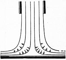
Fig. 166.

§ 165. Distribution of Pressure on a Surface on which a Jet impinges normally.—The principle of momentum gives readily enough the total or resultant pressure of a jet impinging on a plane surface, but in some cases it is useful to know the distribution of the pressure. The problem in the case in which the plane is struck normally, and the jet spreads in all directions, is one of great complexity, but even in that case the maximum intensity of the pressure is easily assigned. Each layer of water flowing from an orifice is gradually deviated (fig. 166) by contact with the surface, and during deviation exercises a centrifugal pressure towards the axis of the jet. The force exerted by each small mass of water is normal to its path and inversely as the radius of curvature of the path. Hence the greatest pressure on the plane must be at the axis of the jet, and the pressure must decrease from the axis outwards, in some such way as is shown by the curve of pressure in fig. 167, the branches of the curve being probably asymptotic to the plane.

For simplicity suppose the jet is a vertical one. Let h1 (fig. 167) be the depth of the orifice from the free surface, and v1 the velocity of discharge. Then, if ω is the area of the orifice, the quantity of water impinging on the plane is obviously

Q = ωv1 = ω √ (2gh1);

that is, supposing the orifice rounded, and neglecting the coefficient of discharge.

The velocity with which the fluid reaches the plane is, however, greater than this, and may reach the value

v = √ (2gh);

where h is the depth of the plane below the free surface. The external layers of fluid subjected throughout, after leaving the orifice, to the atmospheric pressure will attain the velocity v, and will flow away with this velocity unchanged except by friction. The layers towards the interior of the jet, being subjected to a pressure greater than atmospheric pressure, will attain a less velocity, and so much less as they are nearer the centre of the jet. But the pressure can in no case exceed the pressure v2/2g or h measured in feet of water, or the direction of motion of the water would be reversed, and there would be reflux. Hence the maximum intensity of the pressure of the jet on the plane is h ft. of water. If the pressure curve is drawn with pressures represented by feet of water, it will touch the free water surface at the centre of the jet.

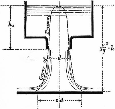
Fig. 167.

Suppose the pressure curve rotated so as to form a solid of revolution. The weight of water contained in that solid is the total pressure of the jet on the surface, which has already been determined. Let V = volume of this solid, then GV is its weight in pounds. Consequently

GV = (G/g) ωv1v; V = 2ω √ (hh1).

We have already, therefore, two conditions to be satisfied by the pressure curve.

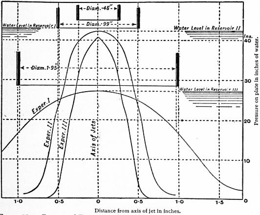
Fig. 168.—Curves of Pressure of Jets impinging normally on a Plane.

Some very interesting experiments on the distribution of pressure on a surface struck by a jet have been made by J. S. Beresford (Prof. Papers on Indian Engineering, No. cccxxii.), with a view to afford information as to the forces acting on the aprons of weirs. Cylindrical jets 1⁄2 in. to 2 in. diameter, issuing from a vessel in which the water level was constant, were allowed to fall vertically on a brass plate 9 in. in diameter. A small hole in the brass plate communicated by a flexible tube with a vertical pressure column. Arrangements were made by which this aperture could be moved 1⁄20 in. at a time across the area struck by the jet. The height of the pressure column, for each position of the aperture, gave the pressure at that point of the area struck by the jet. When the aperture was exactly in the axis of the jet, the pressure column was very nearly level with the free surface in the reservoir supplying the jet; that is, the pressure was very nearly v2/2g. As the aperture moved away from the axis of the jet, the pressure diminished, and it became insensibly small at a distance from the axis of the jet about equal to the diameter of the jet. Hence, roughly, the pressure due to the jet extends over an area about four times the area of section of the jet.

Fig. 168 shows the pressure curves obtained in three experiments with three jets of the sizes shown, and with the free surface level in the reservoir at the heights marked.

Height from Free Surface to Brass Plate in inches. Distance from Axis of Jet in inches. Pressure in inches of Water.

Experiment 1. Jet .475 in. diameter.

43 0 40.5

” .05 39.40

” .1 37.5-39.5

” .15 35

” .2 33.5-37

” .25 31

” .3 21-27

” .35 21

” .4 14

” .45 8

” .5 3.5

” .55 1

” .6 0.5

” .65 0

Experiment 2. Jet .988 in. diameter.

42.15 0 42

” .05 41.9

” .1 41.5-41.8

” .15 41

” .2 40.3

” .25 39.2

” .3 37.5

” .35 34.8

” .45 27

42.25 .5 23

” .55 18.5

” .6 13

” .65 8.3

” .7 5

” .75 3

” .8 2.2

42.15 .85 1.6

” .95 1

Experiment 3. Jet 19.5 in. diameter.

27.15 0 26.9

” .08 26.9

” .13 26.8

” .18 26.5-26.6

” .23 26.4-26.5

” .28 26.3-26.6

27 .33 26.2

” .38 25.9

” .43 25.5

” .48 25

” .53 24.5

” .58 24

” .63 23.3

” .68 22.5

” .73 21.8

” .78 21

” .83 20.3

” .88 19.3

” .93 18

” .98 17

26.5 1.13 13.5

” 1.18 12.5

” 1.23 10.8

” 1.28 9.5

” 1.33 8

” 1.38 7

” 1.43 6.3

” 1.48 5

” 1.53 4.3

” 1.58 3.5

” 1.9 2

As the general form of the pressure curve has been already indicated, it may be assumed that its equation is of the form

y = ab−x2.

But it has already been shown that for x = 0, y = h, hence a = h. To determine the remaining constant, the other condition may be used, that the solid formed by rotating the pressure curve represents the total pressure on the plane. The volume of the solid is

V = ∫∞0 2πxy dx

= 2πh ∫∞0 b−x2x dx

= (πh / loge b) [ −b−x2 ]∞0

= πh / loge b.

Using the condition already stated,

2ω √ (hh1) = πh / loge b, logε b = (π/2ω) √ (h/h1).

Putting the value of b in (2) in eq. (1), and also r for the radius of the jet at the orifice, so that ω = πr2, the equation to the pressure curve is

y = hε−1/2 √(h / h1) (x2 / r2).

§ 166. Resistance of a Plane moving through a Fluid, or Pressure of a Current on a Plane.—When a thin plate moves through the air, or through an indefinitely large mass of still water, in a direction normal to its surface, there is an excess of pressure on the anterior face and a diminution of pressure on the posterior face. Let v be the relative velocity of the plate and fluid, Ω the area of the plate, G the density of the fluid, h the height due to the velocity, then the total resistance is expressed by the equation

R = fGΩv2 / 2g pounds = fGΩh;

where f is a coefficient having about the value 1.3 for a plate moving in still fluid, and 1.8 for a current impinging on a fixed plane, whether the fluid is air or water. The difference in the value of the coefficient in the two cases is perhaps due to errors of experiment. There is a similar resistance to motion in the case of all bodies of “unfair“ form, that is, in which the surfaces over which the water slides are not of gradual and continuous curvature.

The stress between the fluid and plate arises chiefly in this way. The streams of fluid deviated in front of the plate, supposed for definiteness to be moving through the fluid, receive from it forward momentum. Portions of this forward moving water are thrown off laterally at the edges of the plate, and diffused through the surrounding fluid, instead of falling to their original position behind the plate. Other portions of comparatively still water are dragged into motion to fill the space left behind the plate; and there is thus a pressure less than hydrostatic pressure at the back of the plate. The whole resistance to the motion of the plate is the sum of the excess of pressure in front and deficiency of pressure behind. This resistance is independent of any friction or viscosity in the fluid, and is due simply to its inertia resisting a sudden change of direction at the edge of the plate.

Experiments made by a whirling machine, in which the plate is fixed on a long arm and moved circularly, gave the following values of the coefficient f. The method is not free from objection, as the centrifugal force causes a flow outwards across the plate.

Approximate Area of Plate in sq. ft. Values of f.

Borda. Hutton. Thibault.

0.13 1.39 1.24 ..

0.25 1.49 1.43 1.525

0.63 1.64 .. ..

1.11 .. .. 1.784

There is a steady increase of resistance with the size of the plate, in part or wholly due to centrifugal action.

P. L. G. Dubuat (1734-1809) made experiments on a plane 1 ft. square, moved in a straight line in water at 3 to 61⁄2 ft. per second. Calling m the coefficient of excess of pressure in front, and n the coefficient of deficiency of pressure behind, so that f = m + n, he found the following values:—

m = 1; n = 0.433; f = 1.433.

The pressures were measured by pressure columns. Experiments by A. J. Morin (1795-1880), G. Piobert (1793-1871) and I. Didion (1798-1878) on plates of 0.3 to 2.7 sq. ft. area, drawn vertically through water, gave f = 2.18; but the experiments were made in a reservoir of comparatively small depth. For similar plates moved through air they found f = 1.36, a result more in accordance with those which precede.

For a fixed plane in a moving current of water E. Mariotte found f = 1.25. Dubuat, in experiments in a current of water like those mentioned above, obtained the values m = 1.186; n = 0.670; f = 1.856. Thibault exposed to wind pressure planes of 1.17 and 2.5 sq. ft. area, and found f to vary from 1.568 to 2.125, the mean value being f = 1.834, a result agreeing well with Dubuat.

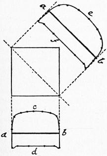
Fig. 169.

§ 167. Stanton’s Experiments on the Pressure of Air on Surfaces.—At the National Physical Laboratory, London, T. E. Stanton carried out a series of experiments on the distribution of pressure on surfaces in a current of air passing through an air trunk. These were on a small scale but with exceptionally accurate means of measurement. These experiments differ from those already given in that the plane is small relatively to the cross section of the current (Proc. Inst. Civ. Eng. clvi., 1904). Fig. 169 shows the distribution of pressure on a square plate. ab is the plate in vertical section. acb the distribution of pressure on the windward and adb that on the leeward side of the central section. Similarly aeb is the distribution of pressure on the windward and afb on the leeward side of a diagonal section. The intensity of pressure at the centre of the plate on the windward side was in all cases p = Gv2/2g ℔ per sq. ft., where G is the weight of a cubic foot of air and v the velocity of the current in ft. per sec. On the leeward side the negative pressure is uniform except near the edges, and its value depends on the form of the plate. For a circular plate the pressure on the leeward side was 0.48 Gv2/2g and for a rectangular plate 0.66 Gv2/2g. For circular or square plates the resultant pressure on the plate was P = 0.00126 v2 ℔ per sq. ft. where v is the velocity of the current in ft. per sec. On a long narrow rectangular plate the resultant pressure was nearly 60% greater than on a circular plate. In later tests on larger planes in free air, Stanton found resistances 18% greater than those observed with small planes in the air trunk.

§ 168. Case when the Direction of Motion is oblique to the Plane.—The determination of the pressure between a fluid and surface in this case is of importance in many practical questions, for instance, in assigning the load due to wind pressure on sloping and curved roofs, and experiments have been made by Hutton, Vince, and Thibault on planes moved circularly through air and water on a whirling machine.

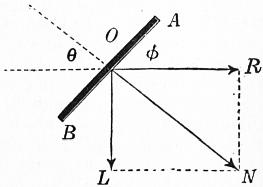
Fig. 170.

Let AB (fig. 170) be a plane moving in the direction R making an angle φ with the plane. The resultant pressure between the fluid and the plane will be a normal pressure N. The component R of this normal pressure is the resistance to the motion of the plane and the other component L is a lateral force resisted by the guides which support the plane. Obviously

R = N sin φ;

L = N cos φ.

In the case of wind pressure on a sloping roof surface, R is the horizontal and L the vertical component of the normal pressure.

In experiments with the whirling machine it is the resistance to motion, R, which is directly measured. Let P be the pressure on a plane moved normally through a fluid. Then, for the same plane inclined at an angle φ to its direction of motion, the resistance was found by Hutton to be

R = P (sin φ)1.842 cos φ.

A simpler and more convenient expression given by Colonel Duchemin is

R = 2P sin2 φ / (1 + sin2 φ).

Consequently, the total pressure between the fluid and plane is

N = 2P sin φ / (1 + sin2 φ) = 2P / (cosec φ + sin φ),

and the lateral force is

L = 2P sin φ cos φ / (1 + sin2 φ).

In 1872 some experiments were made for the Aeronautical Society on the pressure of air on oblique planes. These plates, of 1 to 2 ft. square, were balanced by ingenious mechanism designed by F. H. Wenham and Spencer Browning, in such a manner that both the pressure in the direction of the air current and the lateral force were separately measured. These planes were placed opposite a blast from a fan issuing from a wooden pipe 18 in. square. The pressure of the blast varied from 6⁄10 to 1 in. of water pressure. The following are the results given in pounds per square foot of the plane, and a comparison of the experimental results with the pressures given by Duchemin’s rule. These last values are obtained by taking P = 3.31, the observed pressure on a normal surface:—

Angle between Plane and Direction of Blast 15° 20° 60° 90°

Horizontal pressure R 0.4 0.61 2.73 3.31

Lateral pressure L 1.6 1.96 1.26 ..

Normal pressure √ (L2 + R2) 1.65 2.05 3.01 3.31

Normal pressure by Duchemin’s rule 1.605 2.027 3.276 3.31

Water Motors

In every system of machinery deriving energy from a natural waterfall there exist the following parts:—

1. A supply channel or head race, leading the water from the highest accessible level to the site of the machine. This may be an open channel of earth, masonry or wood, laid at as small a slope as is consistent with the delivery of the necessary supply of water, or it may be a closed cast or wrought-iron pipe, laid at the natural slope of the ground, and about 3 ft. below the surface. In some cases part of the head race is an open channel, part a closed pipe. The channel often starts from a small storage reservoir, constructed near the stream supplying the water motor, in which the water accumulates when the motor is not working. There are sluices or penstocks by which the supply can be cut off when necessary.

2. Leading from the motor there is a tail race, culvert, or discharge pipe delivering the water after it has done its work at the lowest convenient level.

3. A waste channel, weir, or bye-wash is placed at the origin of the head race, by which surplus water, in floods, escapes.

4. The motor itself, of one of the kinds to be described presently, which either overcomes a useful resistance directly, as in the case of a ram acting on a lift or crane chain, or indirectly by actuating transmissive machinery, as when a turbine drives the shafting, belting and gearing of a mill. With the motor is usually combined regulating machinery for adjusting the power and speed to the work done. This may be controlled in some cases by automatic governing machinery.

§ 169. Water Motors with Artificial Sources of Energy.—The great convenience and simplicity of water motors has led to their adoption in certain cases, where no natural source of water power is available. In these cases, an artificial source of water power is created by using a steam-engine to pump water to a reservoir at a great elevation, or to pump water into a closed reservoir in which there is great pressure. The water flowing from the reservoir through hydraulic engines gives back the energy expended, less so much as has been wasted by friction. Such arrangements are most useful where a continuously acting steam engine stores up energy by pumping the water, while the work done by the hydraulic engines is done intermittently.

§ 170. Energy of a Water-fall.—Let Ht be the total fall of level from the point where the water is taken from a natural stream to the point where it is discharged into it again. Of this total fall a portion, which can be estimated independently, is expended in overcoming the resistances of the head and tail races or the supply and discharge pipes. Let this portion of head wasted be ɧr. Then the available head to work the motor is H = Ht − ɧr. It is this available head which should be used in all calculations of the proportions of the motor. Let Q be the supply of water per second. Then GQH foot-pounds per second is the gross available work of the fall. The power of the fall may be utilized in three ways. (a) The GQ pounds of water may be placed on a machine at the highest level, and descending in contact with it a distance of H ft., the work done will be (neglecting losses from friction or leakage) GQH foot-pounds per second. (b) Or the water may descend in a closed pipe from the higher to the lower level, in which case, with the same reservation as before, the pressure at the foot of the pipe will be p = GH pounds per square foot. If the water with this pressure acts on a movable piston like that of a steam engine, it will drive the piston so that the volume described is Q cubic feet per second. Then the work done will be pQ = GHQ foot-pounds per second as before. (c) Or lastly, the water may be allowed to acquire the velocity v = √2gH by its descent. The kinetic energy of Q cubic feet will then be 1⁄2GQv2/g = GQH, and if the water is allowed to impinge on surfaces suitably curved which bring it finally to rest, it will impart to these the same energy as in the previous cases. Motors which receive energy mainly in the three ways described in (a), (b), (c) may be termed gravity, pressure and inertia motors respectively. Generally, if Q ft. per second of water act by weight through a distance h1, at a pressure p due to h2 ft. of fall, and with a velocity v due to h3 ft. of fall, so that h1 + h2 + h3 = H, then, apart from energy wasted by friction or leakage or imperfection of the machine, the work done will be

GQh1 + pQ + (G/g) Q (v2/2g) = GQH foot pounds,

the same as if the water acted simply by its weight while descending H ft.

§ 171. Site for Water Motor.—Wherever a stream flows from a higher to a lower level it is possible to erect a water motor. The amount of power obtainable depends on the available head and the supply of water. In choosing a site the engineer will select a portion of the stream where there is an abrupt natural fall, or at least a considerable slope of the bed. He will have regard to the facility of constructing the channels which are to convey the water, and will take advantage of any bend in the river which enables him to shorten them. He will have accurate measurements made of the quantity of water flowing in the stream, and he will endeavour to ascertain the average quantity available throughout the year, the minimum quantity in dry seasons, and the maximum for which bye-wash channels must be provided. In many cases the natural fall can be increased by a dam or weir thrown across the stream. The engineer will also examine to what extent the head will vary in different seasons, and whether it is necessary to sacrifice part of the fall and give a steep slope to the tail race to prevent the motor being drowned by backwater in floods. Streams fed from lakes which form natural reservoirs or fed from glaciers are less variable than streams depending directly on rainfall, and are therefore advantageous for water-power purposes.

§ 172. Water Power at Holyoke, U.S.A.—About 85 m. from the mouth of the Connecticut river there was a fall of about 60 ft. in a short distance, forming what were called the Grand Rapids, below which the river turned sharply, forming a kind of peninsula on which the city of Holyoke is built. In 1845 the magnitude of the water-power available attracted attention, and it was decided to build a dam across the river. The ordinary flow of the river is 6000 cub. ft. per sec., giving a gross power of 30,000 h.p. In dry seasons the power is 20,000 h.p., or occasionally less. From above the dam a system of canals takes the water to mills on three levels. The first canal starts with a width of 140 ft. and depth of 22 ft., and supplies the highest range of mills. A second canal takes the water which has driven turbines in the highest mills and supplies it to a second series of mills. There is a third canal on a still lower level supplying the lowest mills. The water then finds its way back to the river. With the grant of a mill site is also leased the right to use the water-power. A mill-power is defined as 38 cub. ft. of water per sec. during 16 hours per day on a fall of 20 ft. This gives about 60 h.p. effective. The charge for the power water is at the rate of 20s. per h.p. per annum.