VOLUME XIV SLICE I Husband to Hydrolysis (continued 7)

umean = 0.708 √ {d (p02 − p12)3/2 / ζ l (p03 − p13)}.

(16)

The following table gives some results:—

Absolute Pressures in ℔ per sq. in. Mean Velocities for Tubes of a length in feet.

p0 p1 1000 2000 3000 4000 5000

Vacuum Working 15 5 99.4 70.3 57.4 49.7 44.5

15 10 67.2 47.5 38.8 34.4 30.1

Pressure Working 20 15 57.2 40.5 33.0 28.6 25.6

25 15 74.6 52.7 43.1 37.3 33.3

30 15 84.7 60.0 49.0 42.4 37.9

Limiting Velocity in the Pipe when the Pressure at one End is diminished indefinitely.—If in the last equation there be put p1 = 0, then

u′mean = 0.708 √ (d / ζ l);

where the velocity is independent of the pressure p0 at the other end, a result which apparently must be absurd. Probably for long pipes, as for orifices, there is a limit to the ratio of the initial and terminal pressures for which the formula is applicable.

X. FLOW IN RIVERS AND CANALS

§ 95. Flow of Water in Open Canals and Rivers.—When water flows in a pipe the section at any point is determined by the form of the boundary. When it flows in an open channel with free upper surface, the section depends on the velocity due to the dynamical conditions.

Suppose water admitted to an unfilled canal. The channel will gradually fill, the section and velocity at each point gradually changing. But if the inflow to the canal at its head is constant, the increase of cross section and diminution of velocity at each point attain after a time a limit. Thenceforward the section and velocity at each point are constant, and the motion is steady, or permanent regime is established.

If when the motion is steady the sections of the stream are all equal, the motion is uniform. By hypothesis, the inflow Ωv is constant for all sections, and Ω is constant; therefore v must be constant also from section to section. The case is then one of uniform steady motion. In most artificial channels the form of section is constant, and the bed has a uniform slope. In that case the motion is uniform, the depth is constant, and the stream surface is parallel to the bed. If when steady motion is established the sections are unequal, the motion is steady motion with varying velocity from section to section. Ordinary rivers are in this condition, especially where the flow is modified by weirs or obstructions. Short unobstructed lengths of a river may be treated as of uniform section without great error, the mean section in the length being put for the actual sections.

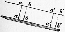
Fig. 102.

In all actual streams the different fluid filaments have different velocities, those near the surface and centre moving faster than those near the bottom and sides. The ordinary formulae for the flow of streams rest on a hypothesis that this variation of velocity may be neglected, and that all the filaments may be treated as having a common velocity equal to the mean velocity of the stream. On this hypothesis, a plane layer abab (fig. 102) between sections normal to the direction of motion is treated as sliding down the channel to a′a′b′b′ without deformation. The component of the weight parallel to the channel bed balances the friction against the channel, and in estimating the friction the velocity of rubbing is taken to be the mean velocity of the stream. In actual streams, however, the velocity of rubbing on which the friction depends is not the mean velocity of the stream, and is not in any simple relation with it, for channels of different forms. The theory is therefore obviously based on an imperfect hypothesis. However, by taking variable values for the coefficient of friction, the errors of the ordinary formulae are to a great extent neutralized, and they may be used without leading to practical errors. Formulae have been obtained based on less restricted hypotheses, but at present they are not practically so reliable, and are more complicated than the formulae obtained in the manner described above.

§ 96. Steady Flow of Water with Uniform Velocity in Channels of Constant Section.—Let aa′, bb′ (fig. 103) be two cross sections normal to the direction of motion at a distance dl. Since the mass aa′bb′ moves uniformly, the external forces acting on it are in equilibrium. Let Ω be the area of the cross sections, χ the wetted perimeter, pq + qr + rs, of a section. Then the quantity m = Ω/χ is termed the hydraulic mean depth of the section. Let v be the mean velocity of the stream, which is taken as the common velocity of all the particles, i, the slope or fall of the stream in feet, per foot, being the ratio bc/ab.

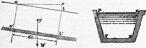
Fig. 103.

The external forces acting on aa′bb′ parallel to the direction of motion are three:—(a) The pressures on aa′ and bb′, which are equal and opposite since the sections are equal and similar, and the mean pressures on each are the same. (b) The component of the weight W of the mass in the direction of motion, acting at its centre of gravity g. The weight of the mass aa′bb′ is GΩ dl, and the component of the weight in the direction of motion is GΩdl × the cosine of the angle between Wg and ab, that is, GΩdl cos abc = GΩ dl bc/ab = GΩidl. (c) There is the friction of the stream on the sides and bottom of the channel. This is proportional to the area χdl of rubbing surface and to a function of the velocity which may be written ƒ(v); ƒ(v) being the friction per sq. ft. at a velocity v. Hence the friction is −χ dl ƒ(v). Equating the sum of the forces to zero,

GΩi dl − χ dl ƒ(v) = 0, ƒ(v) / G = Ωi / χ = mi.

(1)

But it has been already shown (§ 66) that ƒ(v) = ζGv2/2g,

∴ ζv2 / 2g = mi.

(2)

This may be put in the form

v = √ (2g/ζ) √ (mi) = c √ (mi);

(2a)

where c is a coefficient depending on the roughness and form of the channel.

The coefficient of friction ζ varies greatly with the degree of roughness of the channel sides, and somewhat also with the velocity. It must also be made to depend on the absolute dimensions of the section, to eliminate the error of neglecting the variations of velocity in the cross section. A common mean value assumed for ζ is 0.00757. The range of values will be discussed presently.

It is often convenient to estimate the fall of the stream in feet per mile, instead of in feet per foot. If f is the fall in feet per mile,

f = 5280 i.

Putting this and the above value of ζ in (2a), we get the very simple and long-known approximate formula for the mean velocity of a stream—

v = 1⁄4 1⁄2 √ (2mf).

(3)

The flow down the stream per second, or discharge of the stream, is

Q = Ωv = Ωc √ (mi).

(4)

§ 97. Coefficient of Friction for Open Channels.—Various expressions have been proposed for the coefficient of friction for channels as for pipes. Weisbach, giving attention chiefly to the variation of the coefficient of friction with the velocity, proposed an expression of the form

ζ = α (1 + β/v),

(5)

and from 255 experiments obtained for the constants the values

α = 0.007409; β = 0.1920.

This gives the following values at different velocities:—

v = 0.3 0.5 0.7 1 11⁄2 2 3 5 7 10 15

ζ = 0.01215 0.01025 0.00944 0.00883 0.00836 0.00812 0.90788 0.00769 0.00761 0.00755 0.00750

In using this value of ζ when v is not known, it is best to proceed by approximation.

§ 98. Darcy and Bazin’s Expression for the Coefficient of Friction.—Darcy and Bazin’s researches have shown that ζ varies very greatly for different degrees of roughness of the channel bed, and that it also varies with the dimensions of the channel. They give for ζ an empirical expression (similar to that for pipes) of the form

ζ = α (1 + β / m);

(6)

where m is the hydraulic mean depth. For different kinds of channels they give the following values of the coefficient of friction:—

Kind of Channel. α β

I. Very smooth channels, sides of smooth cement or planed timber .00294 0.10

II. Smooth channels, sides of ashlar, brickwork, planks .00373 0.23

III. Rough channels, sides of rubble masonry or pitched with stone .00471 0.82

IV. Very rough canals in earth .00549 4.10

V. Torrential streams encumbered with detritus .00785 5.74

The last values (Class V.) are not Darcy and Bazin’s, but are taken from experiments by Ganguillet and Kutter on Swiss streams.

The following table very much facilitates the calculation of the mean velocity and discharge of channels, when Darcy and Bazin’s value of the coefficient of friction is used. Taking the general formula for the mean velocity already given in equation (2a) above,

v = c √ (mi),

where c = √ (2g/ζ), the following table gives values of c for channels of different degrees of roughness, and for such values of the hydraulic mean depths as are likely to occur in practical calculations:—

Values of c in v = c √ (mi), deduced from Darcy and Bazin’s Values.

Hydraulic Mean. Depth = m. Very Smooth Channels. Cement. Smooth Channels. Ashlar or Brickwork. Rough Channels. Rubble Masonry. Very Rough Channels. Canals in Earth. Excessively Rough Channels encumbered with Detritus.

.25 125 95 57 26 18.5

.5 135 110 72 36 25.6

.75 139 116 81 42 30.8

1.0 141 119 87 48 34.9

1.5 143 122 94 56 41.2

2.0 144 124 98 62 46.0

2.5 145 126 101 67 ..

3.0 145 126 104 70 53

3.5 146 127 105 73 ..

4.0 146 128 106 76 58

4.5 146 128 107 78 ..

5.0 146 128 108 80 62

5.5 146 129 109 82 ..

6.0 147 129 110 84 65

6.5 147 129 110 85 ..

7.0 147 129 110 86 67

7.5 147 129 111 87 ..

8.0 147 130 111 88 69

8.5 147 130 112 89 ..

9.0 147 130 112 90 71

9.5 147 130 112 90 ..

10.0 147 130 112 91 72

11 147 130 113 92 ..

12 147 130 113 93 74

13 147 130 113 94 ..

14 147 130 113 95 ..

15 147 130 114 96 77

16 147 130 114 97 ..

17 147 130 114 97 ..

18 147 130 114 98 ..

20 147 131 114 98 80

25 148 131 115 100 ..

30 148 131 115 102 83

40 148 131 116 103 85

50 148 131 116 104 86

∞ 148 131 117 108 91

§ 99. Ganguillet and Kutter’s Modified Darcy Formula.—Starting from the general expression v = c√mi, Ganguillet and Kutter examined the variations of c for a wider variety of cases than those discussed by Darcy and Bazin. Darcy and Bazin’s experiments were confined to channels of moderate section, and to a limited variation of slope. Ganguillet and Kutter brought into the discussion two very distinct and important additional series of results. The gaugings of the Mississippi by A. A. Humphreys and H. L. Abbot afford data of discharge for the case of a stream of exceptionally large section and or very low slope. On the other hand, their own measurements of the flow in the regulated channels of some Swiss torrents gave data for cases in which the inclination and roughness of the channels were exceptionally great. Darcy and Bazin’s experiments alone were conclusive as to the dependence of the coefficient c on the dimensions of the channel and on its roughness of surface. Plotting values of c for channels of different inclination appeared to indicate that it also depended on the slope of the stream. Taking the Mississippi data only, they found

c = 256 for an inclination of 0.0034 per thousand,

= 154 ” ” 0.02 ”

so that for very low inclinations no constant value of c independent of the slope would furnish good values of the discharge. In small rivers, on the other hand, the values of c vary little with the slope. As regards the influence of roughness of the sides of the channel a different law holds. For very small channels differences of roughness have a great influence on the discharge, but for very large channels different degrees of roughness have but little influence, and for indefinitely large channels the influence of different degrees of roughness must be assumed to vanish. The coefficients given by Darcy and Bazin are different for each of the classes of channels of different roughness, even when the dimensions of the channel are infinite. But, as it is much more probable that the influence of the nature of the sides diminishes indefinitely as the channel is larger, this must be regarded as a defect in their formula.

Comparing their own measurements in torrential streams in Switzerland with those of Darcy and Bazin, Ganguillet and Kutter found that the four classes of coefficients proposed by Darcy and Bazin were insufficient to cover all cases. Some of the Swiss streams gave results which showed that the roughness of the bed was markedly greater than in any of the channels tried by the French engineers. It was necessary therefore in adopting the plan of arranging the different channels in classes of approximately similar roughness to increase the number of classes. Especially an additional class was required for channels obstructed by detritus.

To obtain a new expression for the coefficient in the formula

v = √ (2g / ζ) √ (mi) = c √ (mi),

Ganguillet and Kutter proceeded in a purely empirical way. They found that an expression of the form

c = α / (1 + β/√ m)

could be made to fit the experiments somewhat better than Darcy’s expression. Inverting this, we get

1/c = 1/α + β/α √ m,

an equation to a straight line having 1/√m for abscissa, 1/c for ordinate, and inclined to the axis of abscissae at an angle the tangent of which is β/α.

Plotting the experimental values of 1/c and 1/√ m, the points so found indicated a curved rather than a straight line, so that β must depend on α. After much comparison the following form was arrived at—

c = (A + l/n) / (1 + An / √ m),

where n is a coefficient depending only on the roughness of the sides of the channel, and A and l are new coefficients, the value of which remains to be determined. From what has been already stated, the coefficient c depends on the inclination of the stream, decreasing as the slope i increases.

Let

A = a + p/i.

Then

c = (a + l/n + p/i) / {1 + (a + p/i) n/√ m},

the form of the expression for c ultimately adopted by Ganguillet and Kutter.

For the constants a, l, p Ganguillet and Kutter obtain the values 23, 1 and 0.00155 for metrical measures, or 41.6, 1.811 and 0.00281 for English feet. The coefficient of roughness n is found to vary from 0.008 to 0.050 for either metrical or English measures.

The most practically useful values of the coefficient of roughness n are given in the following table:—

Nature of Sides of Channel. Coefficient of Roughness n.

Well-planed timber 0.009

Cement plaster 0.010

Plaster of cement with one-third sand 0.011

Unplaned planks 0.012

Ashlar and brickwork 0.013

Canvas on frames 0.015

Rubble masonry 0.017

Canals in very firm gravel 0.020

Rivers and canals in perfect order, free from stones or weeds 0.025

Rivers and canals in moderately good order, not quite free from stones and weeds 0.030

Rivers and canals in bad order, with weeds and detritus 0.035

Torrential streams encumbered with detritus 0.050

Ganguillet and Kutter’s formula is so cumbrous that it is difficult to use without the aid of tables.

Lowis D’A. Jackson published complete and extensive tables for facilitating the use of the Ganguillet and Kutter formula (Canal and Culvert Tables, London, 1878). To lessen calculation he puts the formula in this form:—

M = n (41.6 + 0.00281/i);

v = (√ m/n) {(M + 1.811) / (M + √m)} √ (mi).

The following table gives a selection of values of M, taken from Jackson’s tables:—

i Values of M for n =

0.010 0.012 0.015 0.017 0.020 0.025 0.030

.00001 3.2260 3.8712 4.8390 5.4842 6.4520 8.0650 9.6780

.00002 1.8210 2.1852 2.7315 3.0957 3.6420 4.5525 5.4630

.00004 1.1185 1.3422 1.6777 1.9014 2.2370 2.7962 3.3555

.00006 0.8843 1.0612 1.3264 1.5033 1.7686 2.2107 2.6529

.00008 0.7672 0.9206 1.1508 1.3042 1.5344 1.9180 2.3016

.00010 0.6970 0.8364 1.0455 1.1849 1.3940 1.7425 2.0910

.00025 0.5284 0.6341 0.7926 0.8983 1.0568 1.3210 1.5852

.00050 0.4722 0.5666 0.7083 0.8027 0.9444 1.1805 1.4166

.00075 0.4535 0.5442 0.6802 0.7709 0.9070 1.1337 1.3605

.00100 0.4441 0.5329 0.6661 0.7550 0.8882 1.1102 1.3323

.00200 0.4300 0.5160 0.6450 0.7310 0.8600 1.0750 1.2900

.00300 0.4254 0.5105 0.6381 0.7232 0.8508 1.0635 1.2762

A difficulty in the use of this formula is the selection of the coefficient of roughness. The difficulty is one which no theory will overcome, because no absolute measure of the roughness of stream beds is possible. For channels lined with timber or masonry the difficulty is not so great. The constants in that case are few and sufficiently defined. But in the case of ordinary canals and rivers the case is different, the coefficients having a much greater range. For artificial canals in rammed earth or gravel n varies from 0.0163 to 0.0301. For natural channels or rivers n varies from 0.020 to 0.035.

In Jackson’s opinion even Kutter’s numerous classes of channels seem inadequately graduated, and he proposes for artificial canals the following classification:—

I. Canals in very firm gravel, in perfect order n = 0.02

II. Canals in earth, above the average in order n = 0.0225

III. Canals in earth, in fair order n = 0.025

IV. Canals in earth, below the average in order n = 0.0275

V. Canals in earth, in rather bad order, partially overgrown with weeds and obstructed by detritus. n = 0.03

Ganguillet and Kutter’s formula has been considerably used partly from its adoption in calculating tables for irrigation work in India. But it is an empirical formula of an unsatisfactory form. Some engineers apparently have assumed that because it is complicated it must be more accurate than simpler formulae. Comparison with the results of gaugings shows that this is not the case. The term involving the slope was introduced to secure agreement with some early experiments on the Mississippi, and there is strong reason for doubting the accuracy of these results.

§ 100. Bazin’s New Formula.—Bazin subsequently re-examined all the trustworthy gaugings of flow in channels and proposed a modification of the original Darcy formula which appears to be more satisfactory than any hitherto suggested (Étude d’une nouvelle formule, Paris, 1898). He points out that Darcy’s original formula, which is of the form mi/v2 = α + β/m, does not agree with experiments on channels as well as with experiments on pipes. It is an objection to it that if m increases indefinitely the limit towards which mi/v2 tends is different for different values of the roughness. It would seem that if the dimensions of a canal are indefinitely increased the variation of resistance due to differing roughness should vanish. This objection is met if it is assumed that √ (mi/v2) = α + β/√ m, so that if a is a constant mi/v2 tends to the limit a when m increases. A very careful discussion of the results of gaugings shows that they can be expressed more satisfactorily by this new formula than by Ganguillet and Kutter’s. Putting the equation in the form ζv2/2g = mi, ζ = 0.002594 (1 + γ/√ m), where γ has the following values:—

I. Very smooth sides, cement, planed plank, γ = 0.109

II. Smooth sides, planks, brickwork 0.290

III. Rubble masonry sides 0.833

IV. Sides of very smooth earth, or pitching 1.539

V. Canals in earth in ordinary condition 2.353

VI. Canals in earth exceptionally rough 3.168

§ 101. The Vertical Velocity Curve.—If at each point along a vertical representing the depth of a stream, the velocity at that point is plotted horizontally, the curve obtained is the vertical velocity curve and it has been shown by many observations that it approximates to a parabola with horizontal axis. The vertex of the parabola is at the level of the greatest velocity. Thus in fig. 104 OA is the vertical at which velocities are observed; v0 is the surface; vz the maximum and vd the bottom velocity. B C D is the vertical velocity curve which corresponds with a parabola having its vertex at C. The mean velocity at the vertical is

vm = 1⁄3 [2vz + vd + (dz/d) (v0 − vd)].

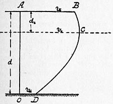
Fig. 104.

The Horizontal Velocity Curve.—Similarly if at each point along a horizontal representing the width of the stream the velocities are plotted, a curve is obtained called the horizontal velocity curve. In streams of symmetrical section this is a curve symmetrical about the centre line of the stream. The velocity varies little near the centre of the stream, but very rapidly near the banks. In unsymmetrical sections the greatest velocity is at the point where the stream is deepest, and the general form of the horizontal velocity curve is roughly similar to the section of the stream.

§ 102. Curves or Contours of Equal Velocity.—If velocities are observed at a number of points at different widths and depths in a stream, it is possible to draw curves on the cross section through points at which the velocity is the same. These represent contours of a solid, the volume of which is the discharge of the stream per second. Fig. 105 shows the vertical and horizontal velocity curves and the contours of equal velocity in a rectangular channel, from one of Bazin’s gaugings.

§ 103. Experimental Observations on the Vertical Velocity Curve.—A preliminary difficulty arises in observing the velocity at a given point in a stream because the velocity rapidly varies, the motion not being strictly steady. If an average of several velocities at the same point is taken, or the average velocity for a sensible period of time, this average is found to be constant. It may be inferred that though the velocity at a point fluctuates about a mean value, the fluctuations being due to eddying motions superposed on the general motion of the stream, yet these fluctuations produce effects which disappear in the mean of a series of observations and, in calculating the volume of flow, may be disregarded.

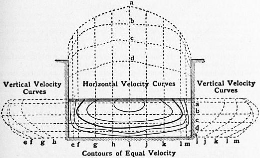
Fig. 105.

In the next place it is found that in most of the best observations on the velocity in streams, the greatest velocity at any vertical is found not at the surface but at some distance below it. In various river gaugings the depth dz at the centre of the stream has been found to vary from 0 to 0.3d.

§ 104. Influence of the Wind.—In the experiments on the Mississippi the vertical velocity curve in calm weather was found to agree fairly with a parabola, the greatest velocity being at 3⁄10ths of the depth of the stream from the surface. With a wind blowing down stream the surface velocity is increased, and the axis of the parabola approaches the surface. On the contrary, with a wind blowing up stream the surface velocity is diminished, and the axis of the parabola is lowered, sometimes to half the depth of the stream. The American observers drew from their observations the conclusion that there was an energetic retarding action at the surface of a stream like that due to the bottom and sides. If there were such a retarding action the position of the filament of maximum velocity below the surface would be explained.

It is not difficult to understand that a wind acting on surface ripples or waves should accelerate or retard the surface motion of the stream, and the Mississippi results may be accepted so far as showing that the surface velocity of a stream is variable when the mean velocity of the stream is constant. Hence observations of surface velocity by floats or otherwise should only be made in very calm weather. But it is very difficult to suppose that, in still air, there is a resistance at the free surface of the stream at all analogous to that at the sides and bottom. Further, in very careful experiments, P. P. Boileau found the maximum velocity, though raised a little above its position for calm weather, still at a considerable distance below the surface, even when the wind was blowing down stream with a velocity greater than that of the stream, and when the action of the air must have been an accelerating and not a retarding action. A much more probable explanation of the diminution of the velocity at and near the free surface is that portions of water, with a diminished velocity from retardation by the sides or bottom, are thrown off in eddying masses and mingle with the rest of the stream. These eddying masses modify the velocity in all parts of the stream, but have their greatest influence at the free surface. Reaching the free surface they spread out and remain there, mingling with the water at that level and diminishing the velocity which would otherwise be found there.

Influence of the Wind on the Depth at which the Maximum Velocity is found.—In the gaugings of the Mississippi the vertical velocity curve was found to agree well with a parabola having a horizontal axis at some distance below the water surface, the ordinate of the parabola at the axis being the maximum velocity of the section. During the gaugings the force of the wind was registered on a scale ranging from 0 for a calm to 10 for a hurricane. Arranging the velocity curves in three sets—(1) with the wind blowing up stream, (2) with the wind blowing down stream, (3) calm or wind blowing across stream—it was found that an upstream wind lowered, and a down-stream wind raised, the axis of the parabolic velocity curve. In calm weather the axis was at 3⁄10ths of the total depth from the surface for all conditions of the stream.

Let h′ be the depth of the axis of the parabola, m the hydraulic mean depth, f the number expressing the force of the wind, which may range from +10 to −10, positive if the wind is up stream, negative if it is down stream. Then Humphreys and Abbot find their results agree with the expression

h′ / m = 0.317 ± 0.06f.

Fig. 106 shows the parabolic velocity curves according to the American observers for calm weather, and for an up- or down-stream wind of a force represented by 4.

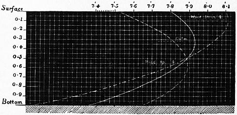
Fig. 106.

It is impossible at present to give a theoretical rule for the vertical velocity curve, but in very many gaugings it has been found that a parabola with horizontal axis fits the observed results fairly well. The mean velocity on any vertical in a stream varies from 0.85 to 0.92 of the surface velocity at that vertical, and on the average if v0 is the surface and vm the mean velocity at a vertical vm = 6⁄7v0, a result useful in float gauging. On any vertical there is a point at which the velocity is equal to the mean velocity, and if this point were known it would be useful in gauging. Humphreys and Abbot in the Mississippi found the mean velocity at 0.66 of the depth; G. H. L. Hagen and H. Heinemann at 0.56 to 0.58 of the depth. The mean of observations by various observers gave the mean velocity at from 0.587 to 0.62 of the depth, the average of all being almost exactly 0.6 of the depth. The mid-depth velocity is therefore nearly equal to, but a little greater than, the mean velocity on a vertical. If vmd is the mid-depth velocity, then on the average vm = 0.98vmd.

§ 105. Mean Velocity on a Vertical from Two Velocity Observations.—A. J. C. Cunningham, in gaugings on the Ganges canal, found the following useful results. Let v0 be the surface, vm the mean, and vxd the velocity at the depth xd; then

vm = 1⁄4 (v0 + 3v2/3d ) = 1⁄2 (v.211d + v.789d ).

§ 106. Ratio of Mean to Greatest Surface Velocity, for the whole Cross Section in Trapezoidal Channels.—It is often very important to be able to deduce the mean velocity, and thence the discharge, from observation of the greatest surface velocity. The simplest method of gauging small streams and channels is to observe the greatest surface velocity by floats, and thence to deduce the mean velocity. In general in streams of fairly regular section the mean velocity for the whole section varies from 0.7 to 0.85 of the greatest surface velocity. For channels not widely differing from those experimented on by Bazin, the expression obtained by him for the ratio of surface to mean velocity may be relied on as at least a good approximation to the truth. Let v0 be the greatest surface velocity, vm the mean velocity of the stream. Then, according to Bazin,

vm = v0 − 25.4 √ (mi).

But

vm = c √ (mi),

where c is a coefficient, the values of which have been already given in the table in § 98. Hence

vm = cv0 / (c + 25.4).

Values of Coefficient c/(c + 25.4) in the Formula vm = cv0/(c + 25.4).

Hydraulic Mean Depth = m. Very Smooth Channels. Cement. Smooth Channels. Ashlar or Brickwork. Rough Channels. Rubble Masonry. Very Rough Channels. Canals in Earth. Channels encumbered with Detritus.

0.25 .83 .79 .69 .51 .42

0.5 .84 .81 .74 .58 .50

0.75 .84 .82 .76 .63 .55

1.0 .85 .. .77 .65 .58

2.0 .. .83 .79 .71 .64

3.0 .. .. .80 .73 .67

4.0 .. .. .81 .75 .70

5.0 .. .. .. .76 .71

6.0 .. .84 .. .77 .72

7.0 .. .. .. .78 .73

8.0 .. .. .. .. ..

9.0 .. .. .82 .. .74

10.0 .. .. .. .. ..

15.0 .. .. .. .79 .75

20.0 .. .. .. .80 .76

30.0 .. .. .82 .. .77

40.0 .. .. .. .. ..

50.0 .. .. .. .. ..

∞ .. .. .. .. .79

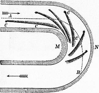
Fig. 107.

§ 107. River Bends.—In rivers flowing in alluvial plains, the windings which already exist tend to increase in curvature by the scouring away of material from the outer bank and the deposition of detritus along the inner bank. The sinuosities sometimes increase till a loop is formed with only a narrow strip of land between the two encroaching branches of the river. Finally a “cut off” may occur, a waterway being opened through the strip of land and the loop left separated from the stream, forming a horseshoe shaped lagoon or marsh. Professor James Thomson pointed out (Proc. Roy. Soc., 1877, p. 356; Proc. Inst. of Mech. Eng., 1879, p. 456) that the usual supposition is that the water tending to go forwards in a straight line rushes against the outer bank and scours it, at the same time creating deposits at the inner bank. That view is very far from a complete account of the matter, and Professor Thomson gave a much more ingenious account of the action at the bend, which he completely confirmed by experiment.

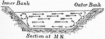
Fig. 108.

When water moves round a circular curve under the action of gravity only, it takes a motion like that in a free vortex. Its velocity is greater parallel to the axis of the stream at the inner than at the outer side of the bend. Hence the scouring at the outer side and the deposit at the inner side of the bend are not due to mere difference of velocity of flow in the general direction of the stream; but, in virtue of the centrifugal force, the water passing round the bend presses outwards, and the free surface in a radial cross section has a slope from the inner side upwards to the outer side (fig. 108). For the greater part of the water flowing in curved paths, this difference of pressure produces no tendency to transverse motion. But the water immediately in contact with the rough bottom and sides of the channel is retarded, and its centrifugal force is insufficient to balance the pressure due to the greater depth at the outside of the bend. It therefore flows inwards towards the inner side of the bend, carrying with it detritus which is deposited at the inner bank. Conjointly with this flow inwards along the bottom and sides, the general mass of water must flow outwards to take its place. Fig. 107 shows the directions of flow as observed in a small artificial stream, by means of light seeds and specks of aniline dye. The lines CC show the directions of flow immediately in contact with the sides and bottom. The dotted line AB shows the direction of motion of floating particles on the surface of the stream.

§ 108. Discharge of a River when flowing at different Depths.—When frequent observations must be made on the flow of a river or canal, the depth of which varies at different times, it is very convenient to have to observe the depth only. A formula can be established giving the flow in terms of the depth. Let Q be the discharge in cubic feet per second; H the depth of the river in some straight and uniform part. Then Q = aH + bH2, where the constants a and b must be found by preliminary gaugings in different conditions of the river. M. C. Moquerey found for part of the upper Saône, Q = 64.7H + 8.2H2 in metric measures, or Q = 696H + 26.8H2 in English measures.

§ 109. Forms of Section of Channels.—The simplest form of section for channels is the semicircular or nearly semicircular channel (fig. 109), a form now often adopted from the facility with which it can be executed in concrete. It has the advantage that the rubbing surface is less in proportion to the area than in any other form.

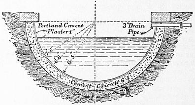
Fig. 109.

Wooden channels or flumes, of which there are examples on a large scale in America, are rectangular in section, and the same form is adopted for wrought and cast-iron aqueducts. Channels built with brickwork or masonry may be also rectangular, but they are often trapezoidal, and are always so if the sides are pitched with masonry laid dry. In a trapezoidal channel, let b (fig. 110) be the bottom breadth, b0 the top breadth, d the depth, and let the slope of the sides be n horizontal to 1 vertical. Then the area of section is Ω = (b + nd) d = (b0 − nd) d, and the wetted perimeter χ = b + 2d √ (n2 + 1).

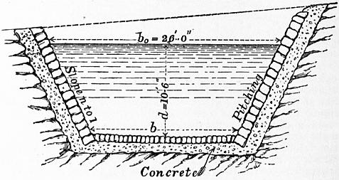
Fig. 110.

When a channel is simply excavated in earth it is always originally trapezoidal, though it becomes more or less rounded in course of time. The slope of the sides then depends on the stability of the earth, a slope of 2 to 1 being the one most commonly adopted.

Figs. 111, 112 show the form of canals excavated in earth, the former being the section of a navigation canal and the latter the section of an irrigation canal.

§ 110. Channels of Circular Section.—The following short table facilitates calculations of the discharge with different depths of water in the channel. Let r be the radius of the channel section; then for a depth of water = κr, the hydraulic mean radius is μr and the area of section of the waterway νr2, where κ, μ, and ν have the following values:—

Depth of water in terms of radius κ = .01 .05 .10 .15 .20 .25 .30 .35 .40 .45 .50 .55 .60 .65 .70 .75 .80 .85 .90 .95 1.0

Hydraulic mean depth in terms of radius μ = .00668 .0321 .0523 .0963 .1278 .1574 .1852 .2142 .242 .269 .293 .320 .343 .365 .387 .408 .429 .449 .466 .484 .500

Waterway in terms of square of radius ν = .00189 .0211 .0598 .1067 .1651 .228 .294 .370 .450 .532 .614 .709 .795 .885 .979 1.075 1.175 1.276 1.371 1.470 1.571

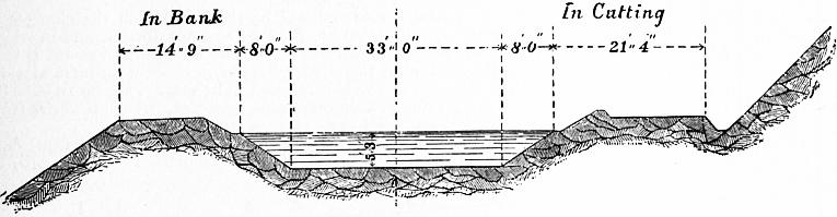
Fig. 111.—Scale 20 ft. = 1 in.

Fig. 112.—Scale 80 ft. = 1 in.

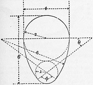
Fig. 113.

§ 111. Egg-Shaped Channels or Sewers.—In sewers for discharging storm water and house drainage the volume of flow is extremely variable; and there is a great liability for deposits to be left when the flow is small, which are not removed during the short periods when the flow is large. The sewer in consequence becomes choked. To obtain uniform scouring action, the velocity of flow should be constant or nearly so; a complete uniformity of velocity cannot be obtained with any form of section suitable for sewers, but an approximation to uniform velocity is obtained by making the sewers of oval section. Various forms of oval have been suggested, the simplest being one in which the radius of the crown is double the radius of the invert, and the greatest width is two-thirds the height. The section of such a sewer is shown in fig. 113, the numbers marked on the figure being proportional numbers.

§ 112. Problems on Channels in which the Flow is Steady and at Uniform Velocity.—The general equations given in §§ 96, 98 are

ζ = α(1 + β/m);

(1)

ζv2/2g = mi;

(2)

Q = Ωv.

(3)

Problem I.—Given the transverse section of stream and discharge, to find the slope. From the dimensions of the section find Ω and m; from (1) find ζ, from (3) find v, and lastly from (2) find i.

Problem II.—Given the transverse section and slope, to find the discharge. Find v from (2), then Q from (3).

Problem III.—Given the discharge and slope, and either the breadth, depth, or general form of the section of the channel, to determine its remaining dimensions. This must generally be solved by approximations. A breadth or depth or both are chosen, and the discharge calculated. If this is greater than the given discharge, the dimensions are reduced and the discharge recalculated.

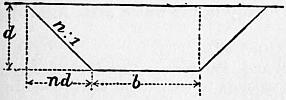
Fig. 114.

Since m lies generally between the limits m = d and m = 1⁄2d, where d is the depth of the stream, and since, moreover, the velocity varies as √ (m) so that an error in the value of m leads only to a much less error in the value of the velocity calculated from it, we may proceed thus. Assume a value for m, and calculate v from it. Let v1 be this first approximation to v. Then Q/v1 is a first approximation to Ω, say Ω1. With this value of Ω design the section of the channel; calculate a second value for m; calculate from it a second value of v, and from that a second value for Ω. Repeat the process till the successive values of m approximately coincide.

§ 113. Problem IV. Most Economical Form of Channel for given Side Slopes.—Suppose the channel is to be trapezoidal in section (fig. 114), and that the sides are to have a given slope. Let the longitudinal slope of the stream be given, and also the mean velocity. An infinite number of channels could be found satisfying the foregoing conditions. To render the problem determinate, let it be remembered that, since for a given discharge Ω∞ √χ, other things being the same, the amount of excavation will be least for that channel which has the least wetted perimeter. Let d be the depth and b the bottom width of the channel, and let the sides slope n horizontal to 1 vertical (fig. 114), then

Ω = (b + nd) d;

χ = b + 2d √ (n2 + 1).

Both Ω and χ are to be minima. Differentiating, and equating to zero.

(db/dd + n) d + b + nd = 0, db/dd + 2 √ (n2 + 1) = 0;

eliminating db/dd,

{n − 2√ (n2 + 1)} d + b + nd = 0; b = 2 {√ (n2 + 1) − n} d.

But

Ω / χ = (b + nd) d / {b + 2d √ (n2 + 1)}.

Inserting the value of b,

m = Ω/χ = {2d √ (n2 + 1) − nd} / {4d √ (n2 + 1) − 2nd} = 1⁄2 d.

That is, with given side slopes, the section is least for a given discharge when the hydraulic mean depth is half the actual depth.

A simple construction gives the form of the channel which fulfils this condition, for it can be shown that when m = 1⁄2d the sides of the channel are tangential to a semicircle drawn on the water line.

Since

Ω / χ = 1⁄2 d,

therefore

Ω = 1⁄2 χd.

(1)

Let ABCD be the channel (fig. 115); from E the centre of AD drop perpendiculars EF, EG, EH on the sides.

Let

AB = CD = a; BC = b; EF = EH = c; and EG = d.

Ω = area AEB + BEC + CED, = ac + 1⁄2 bd.

χ = 2a + b.

Putting these values in (1),

ac + 1⁄2 bd = (a + 1⁄2 b) d; and hence c = d.

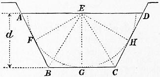
Fig. 115.

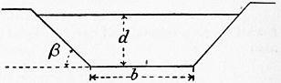
Fig. 116.

That is, EF, EG, EH are all equal, hence a semicircle struck from E with radius equal to the depth of the stream will pass through F and H and be tangential to the sides of the channel.

To draw the channel, describe a semicircle on a horizontal line with radius = depth of channel. The bottom will be a horizontal tangent of that semicircle, and the sides tangents drawn at the required side slopes.

The above result may be obtained thus (fig. 116):—

χ = b + 2d / sin β.

(1)

Ω = d (b + d cot β);

Ω/d = b + d cot β;

(2)

Ω/d2 = b/d + cot β.

(3)

From (1) and (2),

χ = Ω / d − d cot β + 2d / sin β.

This will be a minimum for

dχ / dd = Ω / d2 + cot β − 2 / sin β = 0,

or

Ω/d2 = 2 cosec. β − cot β.

(4)

or

d = √ {Ω sin β / (2 − cos β)}.

From (3) and (4),

b/d = 2 (1 − cos β) / sin β = 2 tan 1⁄2 β.

Proportions of Channels of Maximum Discharge for given Area and Side Slopes. Depth of channel = d; Hydraulic mean depth = 1⁄2d; Area of section = Ω.

Inclination of Sides to Horizon. Ratio of Side Slopes. Area of Section Ω. Bottom Width. Top width = twice length of each Side Slope.

Semicircle .. .. 1.571d2 0 2d

Semi-hexagon 60° 0′ 3 : 5 1.732d2 1.155d 2.310d

Semi-square 90° 0′ 0 : 1 2d2 2d 2d

75° 58′ 1 : 4 1.812d2 1.562d 2.062d

63° 26′ 1 : 2 1.736d2 1.236d 2.236d

53° 8′ 3 : 4 1.750d2 d 2.500d

45° 0′ 1 : 1 1.828d2 0.828d 2.828d

38° 40′ 11⁄4 : 1 1.952d2 0.702d 3.202d

33° 42′ 11⁄2 : 1 2.106d2 0.606d 3.606d

29° 44′ 13⁄4 : 1 2.282d2 0.532d 4.032d

26° 34′ 2 : 1 2.472d2 0.472d 4.472d

23° 58′ 21⁄4 : 1 2.674d2 0.424d 4.924d

21° 48′ 21⁄2 : 1 2.885d2 0.385d 5.385d

19° 58′ 23⁄4 : 1 3.104d2 0.354d 5.854d

18° 26′ 3 : 1 3.325d2 0.325d 6.325d

Half the top width is the length of each side slope. The wetted perimeter is the sum of the top and bottom widths.

§ 114. Form of Cross Section of Channel in which the Mean Velocity is Constant with Varying Discharge.—In designing waste channels from canals, and in some other cases, it is desirable that the mean velocity should be restricted within narrow limits with very different volumes of discharge. In channels of trapezoidal form the velocity increases and diminishes with the discharge. Hence when the discharge is large there is danger of erosion, and when it is small of silting or obstruction by weeds. A theoretical form of section for which the mean velocity would be constant can be found, and, although this is not very suitable for practical purposes, it can be more or less approximated to in actual channels.

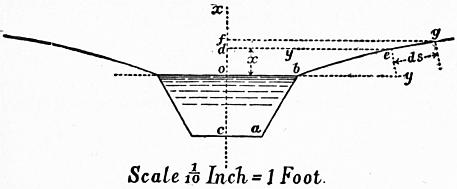
Fig. 117.

Let fig. 117 represent the cross section of the channel. From the symmetry of the section, only half the channel need be considered. Let obac be any section suitable for the minimum flow, and let it be required to find the curve beg for the upper part of the channel so that the mean velocity shall be constant. Take o as origin of coordinates, and let de, fg be two levels of the water above ob.

Let ob = b/2; de = y, fg = y + dy, od = x, of = x + dx; eg = ds.

The condition to be satisfied is that

v = c √ (mi)

should be constant, whether the water-level is at ob, de, or fg. Consequently

m = constant = k

for all three sections, and can be found from the section obac. Hence also

Increment of section = y dx = k.

Increment of perimeter ds

y2 dx2 = k2 ds2 = k2 (dx2 + dy2) and dx = k dy / √ (y2 − k2).

Integrating,

x = k logε {y + √ (y2 − k2)} + constant;

and, since y = b/2 when x = 0,

x = k logε [{y + √ (y2 − k2)} / {1⁄2 b + √ (1⁄4 b2 − k2) }].

Assuming values for y, the values of x can be found and the curve drawn.

The figure has been drawn for a channel the minimum section of which is a half hexagon of 4 ft. depth. Hence k = 2; b = 9.2; the rapid flattening of the side slopes is remarkable.

Steady Motion of Water in Open Channels of Varying Cross Section and Slope

§ 115. In every stream the discharge of which is constant, or may be regarded as constant for the time considered, the velocity at different places depends on the slope of the bed. Except at certain exceptional points the velocity will be greater as the slope of the bed is greater, and, as the velocity and cross section of the stream vary inversely, the section of the stream will be least where the velocity and slope are greatest. If in a stream of tolerably uniform slope an obstruction such as a weir is built, that will cause an alteration of flow similar to that of an alteration of the slope of the bed for a greater or less distance above the weir, and the originally uniform cross section of the stream will become a varied one. In such cases it is often of much practical importance to determine the longitudinal section of the stream.

The cases now considered will be those in which the changes of velocity and cross section are gradual and not abrupt, and in which the only internal work which needs to be taken into account is that due to the friction of the stream bed, as in cases of uniform motion. Further, the motion will be supposed to be steady, the mean velocity at each given cross section remaining constant, though it varies from section to section along the course of the stream.

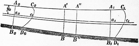
Fig. 118.

Let fig. 118 represent a longitudinal section of the stream, A0A1 being the water surface, B0B1 the stream bed. Let A0B0, A1B1 be cross sections normal to the direction of flow. Suppose the mass of water A0B0A1B1 comes in a short time θ to C0D0C1D1, and let the work done on the mass be equated to its change of kinetic energy during that period. Let l be the length A0A1 of the portion of the stream considered, and z the fall, of surface level in that distance. Let Q be the discharge of the stream per second.

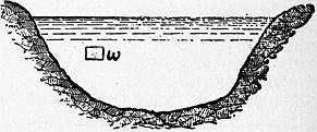
Fig. 119.

Change of Kinetic Energy.—At the end of the time θ there are as many particles possessing the same velocities in the space C0D0A1B1 as at the beginning. The change of kinetic energy is therefore the difference of the kinetic energies of A0B0C0D0 and A1B1C1D1.

Let fig. 119 represent the cross section A0B0, and let ω be a small element of its area at a point where the velocity is v. Let Ω0 be the whole area of the cross section and u0 the mean velocity for the whole cross section. From the definition of mean velocity we have

u0 = Σ ωv / Ω0.

Let v = u0 + w, where w is the difference between the velocity at the small element ω and the mean velocity. For the whole cross section, Σωw = 0.

The mass of fluid passing through the element of section ω, in θ seconds, is (G/g) ωvθ, and its kinetic energy is (G/2g) ωv3θ. For the whole section, the kinetic energy of the mass A0B0C0D0 passing in θ seconds is

(Gθ / 2g) Σωv3 = (Gθ/2g) Σω (u03 + 3u02w + 3u02 + w3), = (Gθ / 2g) {u03Ω + Σωw2 (3u0 + w)}.

The factor 3u0 + w is equal to 2u0 + v, a quantity necessarily positive. Consequently Σωv3 > Ω0u03, and consequently the kinetic energy of A0B0C0D0 is greater than

(Gθ / 2g) Ω0u03 or (Gθ) / 2g) Qu02,

which would be its value if all the particles passing the section had the same velocity u0. Let the kinetic energy be taken at

α (Gθ / 2g) Ω0u03 = α (Gθ / 2g) Qu02,

where α is a corrective factor, the value of which was estimated by J. B. C. J. Bélanger at 1.1.6 Its precise value is not of great importance.

In a similar way we should obtain for the kinetic energy of A1B1C1D1 the expression

α (Gθ / 2g) Ω1u13 = α (Gθ / 2g) Qu12,

where Ω1, u1 are the section and mean velocity at A1B1, and where a may be taken to have the same value as before without any important error.

Hence the change of kinetic energy in the whole mass A0B0A1B1 in θ seconds is

α (Gθ / 2g) Q (u12 − u02).

(1)

Motive Work of the Weight and Pressures.—Consider a small filament a0a1 which comes in θ seconds to c0c1. The work done by gravity during that movement is the same as if the portion a0c0 were carried to a1c1. Let dQ θ be the volume of a0c0 or a1c1, and y0, y1 the depths of a0, a1 from the surface of the stream. Then the volume dQ θ or G dQ θ pounds falls through a vertical height z + y1 − y0, and the work done by gravity is

G dQ θ (z + y1 − y0).

Putting pa for atmospheric pressure, the whole pressure per unit of area at a0 is Gy0 + pa, and that at a1 is −(Gy1 + pa). The work of these pressures is

G (y0 + pa/G − y1 − pa/G) dQ θ = G (y0 − y1) dQ θ.

Adding this to the work of gravity, the whole work is GzdQθ; or, for the whole cross section,

GzQθ.

(2)

Work expended in Overcoming the Friction of the Stream Bed.—Let A′B′, A″B″ be two cross sections at distances s and s + ds from A0B0. Between these sections the velocity may be treated as uniform, because by hypothesis the changes of velocity from section to section are gradual. Hence, to this short length of stream the equation for uniform motion is applicable. But in that case the work in overcoming the friction of the stream bed between A′B′ and A″B″ is

GQθζ (u2 / 2g) (χ / Ω) ds,

where u, χ, Ω are the mean velocity, wetted perimeter, and section at A′B′. Hence the whole work lost in friction from A0B0 to A1B1 will be

GQθ ∫10 ζ (u2 / 2g) (χ / Ω) ds.

(3)

Equating the work given in (2) and (3) to the change of kinetic energy given in (1),

α (GQθ / 2g) (u12 − u02) = GQzθ − GQθ ∫10 ζ (u2 / 2g) (χ / Ω) ds;

∴ z = α (u12 − u02) / 2g + ∫10 ζ (u2 / 2g) (χ / Ω) ds.

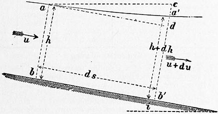
Fig. 120.

§ 116. Fundamental Differential Equation of Steady Varied Motion.—Suppose the equation just found to be applied to an indefinitely short length ds of the stream, limited by the end sections ab, a1b1, taken for simplicity normal to the stream bed (fig. 120). For that short length of stream the fall of surface level, or difference of level of a and a1, may be written dz. Also, if we write u for u0, and u + du for u1, the term (u02 − u12)/2g becomes udu/g. Hence the equation applicable to an indefinitely short length of the stream is

dz = u du/g + (χ/Ω) ζ (u2/2g) ds.

(1)

From this equation some general conclusions may be arrived at as to the form of the longitudinal section of the stream, but, as the investigation is somewhat complicated, it is convenient to simplify it by restricting the conditions of the problem.

Modification of the Formula for the Restricted Case of a Stream flowing in a Prismatic Stream Bed of Constant Slope.—Let i be the constant slope of the bed. Draw ad parallel to the bed, and ac horizontal. Then dz is sensibly equal to a′c. The depths of the stream, h and h + dh, are sensibly equal to ab and a′b′, and therefore dh = a′d. Also cd is the fall of the bed in the distance ds, and is equal to ids. Hence

dz = a′c = cd − a′d = i ds − dh.

(2)

Since the motion is steady—

Q = Ωu = constant.

Differentiating,

Ω du + u dΩ = 0;

∴ du = −u dΩ/Ω.

Let x be the width of the stream, then dΩ = xdh very nearly. Inserting this value,

du = −(ux / Ω) dh.

(3)

Putting the values of du and dz found in (2) and (3) in equation (1),

i ds − dh = −(u2x / gΩ) dh + (χ / Ω) ζ (u2 / 2g) ds.

dh/ds = {i − (χ/Ω) ζ (u2/2g)} / {1 − (u2/g) (x/Ω)}.

(4)

Further Restriction to the Case of a Stream of Rectangular Section and of Indefinite Width.—The equation might be discussed in the form just given, but it becomes a little simpler if restricted in the way just stated. For, if the stream is rectangular, χh = Ω, and if χ is large compared with h, Ω/χ = xh/x = h nearly. Then equation (4) becomes

dh/ds = i (1 − ζu2 / 2gih) / (1 − u2/gh).

(5)

§ 117. General Indications as to the Form of Water Surface furnished by Equation (5).—Let A0A1 (fig. 121) be the water surface, B0B1 the bed in a longitudinal section of the stream, and ab any section at a distance s from B0, the depth ab being h. Suppose B0B1, B0A0 taken as rectangular coordinate axes, then dh/ds is the trigonometric tangent of the angle which the surface of the stream at a makes with the axis B0B1. This tangent dh/ds will be positive, if the stream is increasing in depth in the direction B0B1; negative, if the stream is diminishing in depth from B0 towards B1. If dh/ds = 0, the surface of the stream is parallel to the bed, as in cases of uniform motion. But from equation (4)

dh/ds = 0, if i − (χ/Ω) ζ (u2/2g) = 0;

∴ ζ (u2/2g) = (Ω/χ) i = mi,

which is the well-known general equation for uniform motion, based on the same assumptions as the equation for varied steady motion now being considered. The case of uniform motion is therefore a limiting case between two different kinds of varied motion.

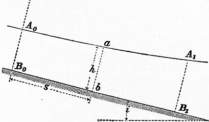
Fig. 121.

Consider the possible changes of value of the fraction

(1 − ζu2 / 2gih) / (1 − u2 / gh).

As h tends towards the limit 0, and consequently u is large, the numerator tends to the limit −∞. On the other hand if h = ∞, in which case u is small, the numerator becomes equal to 1. For a value H of h given by the equation

1 − ζu2 / 2giH = 0, H = ζu2 / 2gi,

we fall upon the case of uniform motion. The results just stated may be tabulated thus:—

For h = 0, H, > H, ∞,

the numerator has the value −∞, 0, > 0, 1.

Next consider the denominator. If h becomes very small, in which case u must be very large, the denominator tends to the limit −∞. As h becomes very large and u consequently very small, the denominator tends to the limit 1. For h = u2/g, or u = √ (gh), the denominator becomes zero. Hence, tabulating these results as before:—

For h = 0, u2/g, > u2/g, ∞,

the denominator becomes −∞, 0, > 0, 1.

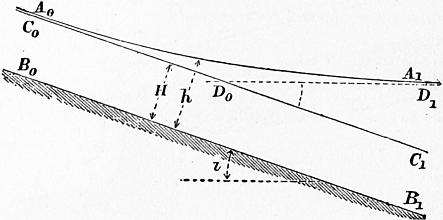
Fig. 122.

§ 118. Case 1.—Suppose h > u2/g, and also h > H, or the depth greater than that corresponding to uniform motion. In this case dh/ds is positive, and the stream increases in depth in the direction of flow. In fig. 122 let B0B1 be the bed, C0C1 a line parallel to the bed and at a height above it equal to H. By hypothesis, the surface A0A1 of the stream is above C0C1, and it has just been shown that the depth of the stream increases from B0 towards B1. But going up stream h approaches more and more nearly the value H, and therefore dh/ds approaches the limit 0, or the surface of the stream is asymptotic to C0C1. Going down stream h increases and u diminishes, the numerator and denominator of the fraction (1 − ζu2/2gih) / (1 − u2/gh) both tend towards the limit 1, and dh/ds to the limit i. That is, the surface of the stream tends to become asymptotic to a horizontal line D0D1.

The form of water surface here discussed is produced when the flow of a stream originally uniform is altered by the construction of a weir. The raising of the water surface above the level C0C1 is termed the backwater due to the weir.

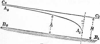
Fig. 123.

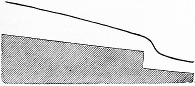
Fig. 124.

§ 119. Case 2.—Suppose h > u2/g, and also h < H. Then dh/ds is negative, and the stream is diminishing in depth in the direction of flow. In fig. 123 let B0B1 be the stream bed as before; C0C1 a line drawn parallel to B0B1 at a height above it equal to H. By hypothesis the surface A0A1 of the stream is below C0C1, and the depth has just been shown to diminish from B0 towards B1. Going up stream h approaches the limit H, and dh/ds tends to the limit zero. That is, up stream A0A1 is asymptotic to C0C1. Going down stream h diminishes and u increases; the inequality h > u2/g diminishes; the denominator of the fraction (1 − ζu2/2gih) / (1 − u2/gh) tends to the limit zero, and consequently dh/ds tends to ∞. That is, down stream A0A1 tends to a direction perpendicular to the bed. Before, however, this limit was reached the assumptions on which the general equation is based would cease to be even approximately true, and the equation would cease to be applicable. The filaments would have a relative motion, which would make the influence of internal friction in the fluid too important to be neglected. A stream surface of this form may be produced if there is an abrupt fall in the bed of the stream (fig. 124).

On the Ganges canal, as originally constructed, there were abrupt falls precisely of this kind, and it appears that the lowering of the water surface and increase of velocity which such falls occasion, for a distance of some miles up stream, was not foreseen. The result was that, the velocity above the falls being greater than was intended, the bed was scoured and considerable damage was done to the works. “When the canal was first opened the water was allowed to pass freely over the crests of the overfalls, which were laid on the level of the bed of the earthen channel; erosion of bed and sides for some miles up rapidly followed, and it soon became apparent that means must be adopted for raising the surface of the stream at those points (that is, the crests of the falls). Planks were accordingly fixed in the grooves above the bridge arches, or temporary weirs were formed over which the water was allowed to fall; in some cases the surface of the water was thus raised above its normal height, causing a backwater in the channel above” (Crofton’s Report on the Ganges Canal, p. 14). Fig. 125 represents in an exaggerated form what probably occurred, the diagram being intended to represent some miles’ length of the canal bed above the fall. AA parallel to the canal bed is the level corresponding to uniform motion with the intended velocity of the canal. In consequence of the presence of the ogee fall, however, the water surface would take some such form as BB, corresponding to Case 2 above, and the velocity would be greater than the intended velocity, nearly in the inverse ratio of the actual to the intended depth. By constructing a weir on the crest of the fall, as shown by dotted lines, a new water surface CC corresponding to Case 1 would be produced, and by suitably choosing the height of the weir this might be made to agree approximately with the intended level AA.

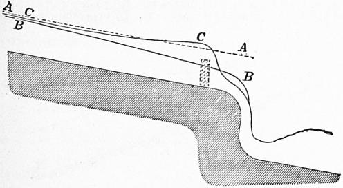
Fig. 125.

§ 120. Case 3.—Suppose a stream flowing uniformly with a depth h < u2/g. For a stream in uniform motion ζu2/2g = mi, or if the stream is of indefinitely great width, so that m = H, then ζu2/2g = iH, and H = ζu2/2gi. Consequently the condition stated above involves that

ζu2 / 2gi < u2 / g, or that i > ζ/2.

If such a stream is interfered with by the construction of a weir which raises its level, so that its depth at the weir becomes h1 > u2/g, then for a portion of the stream the depth h will satisfy the conditions h < u2/g and h > H, which are not the same as those assumed in the two previous cases. At some point of the stream above the weir the depth h becomes equal to u2/g, and at that point dh/ds becomes infinite, or the surface of the stream is normal to the bed. It is obvious that at that point the influence of internal friction will be too great to be neglected, and the general equation will cease to represent the true conditions of the motion of the water. It is known that, in cases such as this, there occurs an abrupt rise of the free surface of the stream, or a standing wave is formed, the conditions of motion in which will be examined presently.

It appears that the condition necessary to give rise to a standing wave is that i > ζ/2. Now ζ depends for different channels on the roughness of the channel and its hydraulic mean depth. Bazin calculated the values of ζ for channels of different degrees of roughness and different depths given in the following table, and the corresponding minimum values of i for which the exceptional case of the production of a standing wave may occur.

Nature of Bed of Stream. Slope below which a Standing Wave is impossible in feet peer foot. Standing Wave Formed.

Slope in feet per foot. Least Depth in feet.

Very smooth cemented surface 0.00147 0.002 0.262

0.003 .098

0.004 .065

Ashlar or brickwork 0.00186 0.003 .394

0.004 .197

0.006 .098

Rubble masonry 0.00235 0.004 1.181

0.006 .525

0.010 .262

Earth 0.00275 0.006 3.478

0.010 1.542

0.015 .919

Standing Waves

§ 121. The formation of a standing wave was first observed by Bidone. Into a small rectangular masonry channel, having a slope of 0.023 ft. per foot, he admitted water till it flowed uniformly with a depth of 0.2 ft. He then placed a plank across the stream which raised the level just above the obstruction to 0.95 ft. He found that the stream above the obstruction was sensibly unaffected up to a point 15 ft. from it. At that point the depth suddenly increased from 0.2 ft. to 0.56 ft. The velocity of the stream in the part unaffected by the obstruction was 5.54 ft. per second. Above the point where the abrupt change of depth occurred u2 = 5.542 = 30.7, and gh = 32.2 × 0.2 = 6.44; hence u2 was > gh. Just below the abrupt change of depth u = 5.54 × 0.2/0.56 = 1.97; u2 = 3.88; and gh = 32.2 × 0.56 = 18.03; hence at this point u2 < gh. Between these two points, therefore, u2 = gh; and the condition for the production of a standing wave occurred.

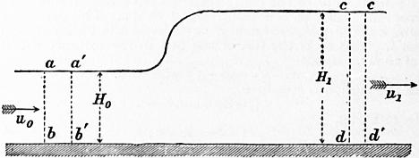
Fig. 126.

The change of level at a standing wave may be found thus. Let fig. 126 represent the longitudinal section of a stream and ab, cd cross sections normal to the bed, which for the short distance considered may be assumed horizontal. Suppose the mass of water abcd to come to a′b′c′d′ in a short time t; and let u0, u1 be the velocities at ab and cd, Ω0, Ω1 the areas of the cross sections. The force causing change of momentum in the mass abcd estimated horizontally is simply the difference of the pressures on ab and cd. Putting h0, h1 for the depths of the centres of gravity of ab and cd measured down from the free water surface, the force is G (h0Ω0 − h1Ω1) pounds, and the impulse in t seconds is G (h0Ω0 − h1Ω1) t second pounds. The horizontal change of momentum is the difference of the momenta of cdc′d′ and aba′b′; that is,

(G/g) (Ω1u12 − Ω0u02) t.

Hence, equating impulse and change of momentum,

G (h0Ω0 − h1Ω1) t = (G/g) (Ω1u12 − Ω0u02) t;

∴ h0Ω0 − h1Ω1 = (Ω1u12 − Ω0u02) / g.

(1)

For simplicity let the section be rectangular, of breadth B and depths H0 and H1, at the two cross sections considered; then h0 = 1⁄2H0, and h1 = 1⁄2H1. Hence

H02 − H12 = (2/g) (H1u12 − H0u02).

But, since Ω0u0 = Ω1u1, we have

u12 = u02H02 / H12,

H02 − H12 = (2u02/g) (H02/H1 − H0).

(2)

This equation is satisfied if H0 = H1, which corresponds to the case of uniform motion. Dividing by H0 − H1, the equation becomes

(H1/H0) (H0 + H1) = 2u02 / g;

(3)

∴ H1 = √ (2u02H0 / g + 1⁄4 H02) − 1⁄2 H0.

(4)

In Bidone’s experiment u0 = 5.54, and H0 = 0.2. Hence H1 = 0.52, which agrees very well with the observed height.

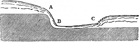
Fig. 127.

§ 122. A standing wave is frequently produced at the foot of a weir. Thus in the ogee falls originally constructed on the Ganges canal a standing wave was observed as shown in fig. 127. The water falling over the weir crest A acquired a very high velocity on the steep slope AB, and the section of the stream at B became very small. It easily happened, therefore, that at B the depth h < u2/g. In flowing along the rough apron of the weir the velocity u diminished and the depth h increased. At a point C, where h became equal to u2/g, the conditions for producing the standing wave occurred. Beyond C the free surface abruptly rose to the level corresponding to uniform motion with the assigned slope of the lower reach of the canal.

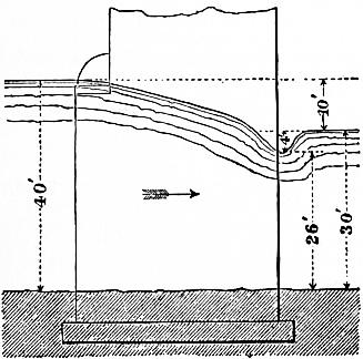
Fig. 128.

A standing wave is sometimes formed on the down stream side of bridges the piers of which obstruct the flow of the water. Some interesting cases of this kind are described in a paper on the “Floods in the Nerbudda Valley” in the Proc. Inst. Civ. Eng. vol. xxvii. p. 222, by A. C. Howden. Fig. 128 is compiled from the data given in that paper. It represents the section of the stream at pier 8 of the Towah Viaduct, during the flood of 1865. The ground level is not exactly given by Howden, but has been inferred from data given on another drawing. The velocity of the stream was not observed, but the author states it was probably the same as at the Gunjal river during a similar flood, that is 16.58 ft. per second. Now, taking the depth on the down stream face of the pier at 26 ft., the velocity necessary for the production of a standing wave would be u = √ (gh) = √ (32.2 × 26) = 29 ft. per second nearly. But the velocity at this point was probably from Howden’s statements 16.58 × 40⁄26 = 25.5 ft. per second, an agreement as close as the approximate character of the data would lead us to expect.

XI. ON STREAMS AND RIVERS

§ 123. Catchment Basin.—A stream or river is the channel for the discharge of the available rainfall of a district, termed its catchment basin. The catchment basin is surrounded by a ridge or watershed line, continuous except at the point where the river finds an outlet. The area of the catchment basin may be determined from a suitable contoured map on a scale of at least 1 in 100,000. Of the whole rainfall on the catchment basin, a part only finds its way to the stream. Part is directly re-evaporated, part is absorbed by vegetation, part may escape by percolation into neighbouring districts. The following table gives the relation of the average stream discharge to the average rainfall on the catchment basin (Tiefenbacher).

Ratio of average Discharge to average Rainfall. Loss by Evaporation, &c., in per cent of total Rainfall.

Cultivated land and spring-forming declivities. 3 to .33 67 to 70

Wooded hilly slopes. .35 to .45 55 to 65

Naked unfissured mountains .55 to .60 40 to 45

§ 124. Flood Discharge.—The flood discharge can generally only be determined by examining the greatest height to which floods have been known to rise. To produce a flood the rainfall must be heavy and widely distributed, and to produce a flood of exceptional height the duration of the rainfall must be so great that the flood waters of the most distant affluents reach the point considered, simultaneously with those from nearer points. The larger the catchment basin the less probable is it that all the conditions tending to produce a maximum discharge should simultaneously occur. Further, lakes and the river bed itself act as storage reservoirs during the rise of water level and diminish the rate of discharge, or serve as flood moderators. The influence of these is often important, because very heavy rain storms are in most countries of comparatively short duration. Tiefenbacher gives the following estimate of the flood discharge of streams in Europe:—

Flood discharge of Streams per Second per Square Mile of Catchment Basin.

In flat country 8.7 to 12.5 cub. ft.

In hilly districts 17.5 to 22.5 ”

In moderately mountainous districts 36.2 to 45.0 ”

In very mountainous districts 50.0 to 75.0 ”

It has been attempted to express the decrease of the rate of flood discharge with the increase of extent of the catchment basin by empirical formulae. Thus Colonel P. P. L. O’Connell proposed the formula y = M √ x, where M is a constant called the modulus of the river, the value of which depends on the amount of rainfall, the physical characters of the basin, and the extent to which the floods are moderated by storage of the water. If M is small for any given river, it shows that the rainfall is small, or that the permeability or slope of the sides of the valley is such that the water does not drain rapidly to the river, or that lakes and river bed moderate the rise of the floods. If values of M are known for a number of rivers, they may be used in inferring the probable discharge of other similar rivers. For British rivers M varies from 0.43 for a small stream draining meadow land to 37 for the Tyne. Generally it is about 15 or 20. For large European rivers M varies from 16 for the Seine to 67.5 for the Danube. For the Nile M = 11, a low value which results from the immense length of the Nile throughout which it receives no affluent, and probably also from the influence of lakes. For different tributaries of the Mississippi M varies from 13 to 56. For various Indian rivers it varies from 40 to 303, this variation being due to the great variations of rainfall, slope and character of Indian rivers.

In some of the tank projects in India, the flood discharge has been calculated from the formula D = C3√ n2, where D is the discharge in cubic yards per hour from n square miles of basin. The constant C was taken = 61,523 in the designs for the Ekrooka tank, = 75,000 on Ganges and Godavery works, and = 10,000 on Madras works.

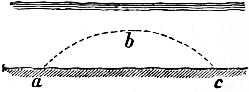
Fig. 129.

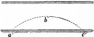
Fig. 130.

§ 125. Action of a Stream on its Bed.—If the velocity of a stream exceeds a certain limit, depending on its size, and on the size, heaviness, form and coherence of the material of which its bed is composed, it scours its bed and carries forward the materials. The quantity of material which a given stream can carry in suspension depends on the size and density of the particles in suspension, and is greater as the velocity of the stream is greater. If in one part of its course the velocity of a stream is great enough to scour the bed and the water becomes loaded with silt, and in a subsequent part of the river’s course the velocity is diminished, then part of the transported material must be deposited. Probably deposit and scour go on simultaneously over the whole river bed, but in some parts the rate of scour is in excess of the rate of deposit, and in other parts the rate of deposit is in excess of the rate of scour. Deep streams appear to have the greatest scouring power at any given velocity. It is possible that the difference is strictly a difference of transporting, not of scouring action. Let fig. 129 represent a section of a stream. The material lifted at a will be diffused through the mass of the stream and deposited at different distances down stream. The average path of a particle lifted at a will be some such curve as abc, and the average distance of transport each time a particle is lifted will be represented by ac. In a deeper stream such as that in fig. 130, the average height to which particles are lifted, and, since the rate of vertical fall through the water may be assumed the same as before, the average distance a′c′ of transport will be greater. Consequently, although the scouring action may be identical in the two streams, the velocity of transport of material down stream is greater as the depth of the stream is greater. The effect is that the deep stream excavates its bed more rapidly than the shallow stream.

§ 126. Bottom Velocity at which Scour commences.—The following bottom velocities were determined by P. L. G. Dubuat to be the maximum velocities consistent with stability of the stream bed for different materials.

Darcy and Bazin give, for the relation of the mean velocity vm and bottom velocity vb.

vm = vb + 10.87 √ (mi).

But

√ mi = vm √ (ζ / 2g);

∴ vm = vb / (1 − 10.87 √ (ζ / 2g)).

Taking a mean value for ζ, we get

vm = 1.312 vb,

and from this the following values of the mean velocity are obtained:—

Bottom Velocity = vb. Mean Velocity = vm.

1. Soft earth 0.25 .33

2. Loam 0.50 .65

3. Sand 1.00 1.30

4. Gravel 2.00 2.62

5. Pebbles 3.40 4.46

6. Broken stone, flint 4.00 5.25

7. Chalk, soft shale 5.00 6.56

8. Rock in beds 6.00 7.87

9. Hard rock. 10.00 13.12

The following table of velocities which should not be exceeded in channels is given in the Ingenieurs Taschenbuch of the Verein “Hütte”:—

Surface Velocity. Mean Velocity. Bottom Velocity.

Slimy earth or brown clay .49 .36 .26

Clay .98 .75 .52

Firm sand 1.97 1.51 1.02

Pebbly bed 4.00 3.15 2.30

Boulder bed 5.00 4.03 3.08

Conglomerate of slaty fragments 7.28 6.10 4.90

Stratified rocks 8.00 7.45 6.00

Hard rocks 14.00 12.15 10.36

§ 127. Regime of a River Channel.—A river channel is said to be in a state of regime, or stability, when it changes little in draught or form in a series of years. In some rivers the deepest part of the channel changes its position perpetually, and is seldom found in the same place in two successive years. The sinuousness of the river also changes by the erosion of the banks, so that in time the position of the river is completely altered. In other rivers the change from year to year is very small, but probably the regime is never perfectly stable except where the rivers flow over a rocky bed.

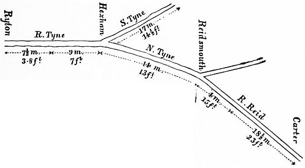
Fig. 131.

If a river had a constant discharge it would gradually modify its bed till a permanent regime was established. But as the volume discharged is constantly changing, and therefore the velocity, silt is deposited when the velocity decreases, and scour goes on when the velocity increases in the same place. When the scouring and silting are considerable, a perfect balance between the two is rarely established, and hence continual variations occur in the form of the river and the direction of its currents. In other cases, where the action is less violent, a tolerable balance may be established, and the deepening of the bed by scour at one time is compensated by the silting at another. In that case the general regime is permanent, though alteration is constantly going on. This is more likely to happen if by artificial means the erosion of the banks is prevented. If a river flows in soil incapable of resisting its tendency to scour it is necessarily sinuous (§ 107), for the slightest deflection of the current to either side begins an erosion which increases progressively till a considerable bend is formed. If such a river is straightened it becomes sinuous again unless its banks are protected from scour.

§ 128. Longitudinal Section of River Bed.—The declivity of rivers decreases from source to mouth. In their higher parts rapid and torrential, flowing over beds of gravel or boulders, they enlarge in volume by receiving affluent streams, their slope diminishes, their bed consists of smaller materials, and finally they reach the sea. Fig. 131 shows the length in miles, and the surface fall in feet per mile, of the Tyne and its tributaries.

The decrease of the slope is due to two causes. (1) The action of the transporting power of the water, carrying the smallest debris the greatest distance, causes the bed to be less stable near the mouth than in the higher parts of the river; and, as the river adjusts its slope to the stability of the bed by scouring or increasing its sinuousness when the slope is too great, and by silting or straightening its course if the slope is too small, the decreasing stability of the bed would coincide with a decreasing slope. (2) The increase of volume and section of the river leads to a decrease of slope; for the larger the section the less slope is necessary to ensure a given velocity.

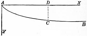
Fig. 132.

The following investigation, though it relates to a purely arbitrary case, is not without interest. Let it be assumed, to make the conditions definite—(1) that a river flows over a bed of uniform resistance to scour, and let it be further assumed that to maintain stability the velocity of the river in these circumstances is constant from source to mouth; (2) suppose the sections of the river at all points are similar, so that, b being the breadth of the river at any point, its hydraulic mean depth is ab and its section is cb2, where a and c are constants applicable to all parts of the river; (3) let us further assume that the discharge increases uniformly in consequence of the supply from affluents, so that, if l is the length of the river from its source to any given point, the discharge there will be kl, where k is another constant applicable to all points in the course of the river.

Let AB (fig. 132) be the longitudinal section of the river, whose source is at A; and take A for the origin of vertical and horizontal coordinates. Let C be a point whose ordinates are x and y, and let the river at C have the breadth b, the slope i, and the velocity v.

Since velocity × area of section = discharge, vcb2 = kl, or b = √ (kl/cv).

Hydraulic mean depth = ab = a √ (kl/cv).

But, by the ordinary formula for the flow of rivers, mi = ζv2;

∴ i = ζv2 / m = (ζv5/2 / a) √ (c / kl).

But i is the tangent of the angle which the curve at C makes with the axis of X, and is therefore = dy/dx. Also, as the slope is small, l = AC = AD = x nearly.

∴ dy/dx = (ζv5/2 / a) √ (c / kx);

and, remembering that v is constant,

y = (2ζv5/2 / a) √ (cx / k);

or

y2 = constant × x;

so that the curve is a common parabola, of which the axis is horizontal and the vertex at the source. This may be considered an ideal longitudinal section, to which actual rivers approximate more or less, with exceptions due to the varying hardness of their beds, and the irregular manner in which their volume increases.

§ 129. Surface Level of River.—The surface level of a river is a plane changing constantly in position from changes in the volume of water discharged, and more slowly from changes in the river bed, and the circumstances affecting the drainage into the river.

For the purposes of the engineer, it is important to determine (1) the extreme low water level, (2) the extreme high water or flood level, and (3) the highest navigable level.

1. Low Water Level cannot be absolutely known, because a river reaches its lowest level only at rare intervals, and because alterations in the cultivation of the land, the drainage, the removal of forests, the removal or erection of obstructions in the river bed, &c., gradually alter the conditions of discharge. The lowest level of which records can be found is taken as the conventional or approximate low water level, and allowance is made for possible changes.

2. High Water or Flood Level.—The engineer assumes as the highest flood level the highest level of which records can be obtained. In forming a judgment of the data available, it must be remembered that the highest level at one point of a river is not always simultaneous with the attainment of the highest level at other points, and that the rise of a river in flood is very different in different parts of its course. In temperate regions, the floods of rivers seldom rise more than 20 ft. above low-water level, but in the tropics the rise of floods is greater.

3. Highest Navigable Level.—When the river rises above a certain level, navigation becomes difficult from the increase of the velocity of the current, or from submersion of the tow paths, or from the headway under bridges becoming insufficient. Ordinarily the highest navigable level may be taken to be that at which the river begins to overflow its banks.

§ 130. Relative Value of Different Materials for Submerged Works.—That the power of water to remove and transport different materials depends on their density has an important bearing on the selection of materials for submerged works. In many cases, as in the aprons or floorings beneath bridges, or in front of locks or falls, and in the formation of training walls and breakwaters by pierres perdus, which have to resist a violent current, the materials of which the structures are composed should be of such a size and weight as to be able individually to resist the scouring action of the water. The heaviest materials will therefore be the best; and the different value of materials in this respect will appear much more striking, if it is remembered that all materials lose part of their weight in water. A block whose volume is V cubic feet, and whose density in air is w ℔ per cubic foot, weighs in air wV ℔, but in water only (w—62.4) V ℔.

Weight of a Cub. Ft. in ℔.

In Air. In Water.

Basalt 187.3 124.9

Brick 130.0 67.6

Brickwork 112.0 49.6

Granite and limestone 170.0 107.6

Sandstone 144.0 81.6

Masonry 116-144 53.6-81.6

§ 131. Inundation Deposits from a River.—When a river carrying silt periodically overflows its banks, it deposits silt over the area flooded, and gradually raises the surface of the country. The silt is deposited in greatest abundance where the water first leaves the river. It hence results that the section of the country assumes a peculiar form, the river flowing in a trough along the crest of a ridge, from which the land slopes downwards on both sides. The silt deposited from the water forms two wedges, having their thick ends towards the river (fig. 133).

Fig. 133.

This is strikingly the case with the Mississippi, and that river is now kept from flooding immense areas by artificial embankments or levees. In India, the term deltaic segment is sometimes applied to that portion of a river running through deposits formed by inundation, and having this characteristic section. The irrigation of the country in this case is very easy; a comparatively slight raising of the river surface by a weir or annicut gives a command of level which permits the water to be conveyed to any part of the district.

§ 132. Deltas.—The name delta was originally given to the Δ-shaped portion of Lower Egypt, included between seven branches of the Nile. It is now given to the whole of the alluvial tracts round river mouths formed by deposition of sediment from the river, where its velocity is checked on its entrance to the sea. The characteristic feature of these alluvial deltas is that the river traverses them, not in a single channel, but in two or many bifurcating branches. Each branch has a tract of the delta under its influence, and gradually raises the surface of that tract, and extends it seaward. As the delta extends itself seaward, the conditions of discharge through the different branches change. The water finds the passage through one of the branches less obstructed than through the others; the velocity and scouring action in that branch are increased; in the others they diminish. The one channel gradually absorbs the whole of the water supply, while the other branches silt up. But as the mouth of the new main channel extends seaward the resistance increases both from the greater length of the channel and the formation of shoals at its mouth, and the river tends to form new bifurcations AC or AD (fig. 134), and one of these may in time become the main channel of the river.

§ 133. Field Operations preliminary to a Study of River Improvement.—There are required (1) a plan of the river, on which the positions of lines of levelling and cross sections are marked; (2) a longitudinal section and numerous cross sections of the river; (3) a series of gaugings of the discharge at different points and in different conditions of the river.

Longitudinal Section.—This requires to be carried out with great accuracy. A line of stakes is planted, following the sinuosities of the river, and chained and levelled. The cross sections are referred to the line of stakes, both as to position and direction. The determination of the surface slope is very difficult, partly from its extreme smallness, partly from oscillation of the water. Cunningham recommends that the slope be taken in a length of 2000 ft. by four simultaneous observations, two on each side of the river.

Fig. 134.

§ 134. Cross Sections—A stake is planted flush with the water, and its level relatively to some point on the line of levels is determined. Then the depth of the water is determined at a series of points (if possible at uniform distances) in a line starting from the stake and perpendicular to the thread of the stream. To obtain these, a wire may be stretched across with equal distances marked on it by hanging tags. The depth at each of these tags may be obtained by a light wooden staff, with a disk-shaped shoe 4 to 6 in. in diameter. If the depth is great, soundings may be taken by a chain and weight. To ensure the wire being perpendicular to the thread of the stream, it is desirable to stretch two other wires similarly graduated, one above and the other below, at a distance of 20 to 40 yds. A number of floats being then thrown in, it is observed whether they pass the same graduation on each wire.

Fig. 135.

For large and rapid rivers the cross section is obtained by sounding in the following way. Let AC (fig. 135) be the line on which soundings are required. A base line AB is measured out at right angles to AC, and ranging staves are set up at AB and at D in line with AC. A boat is allowed to drop down stream, and, at the moment it comes in line with AD, the lead is dropped, and an observer in the boat takes, with a box sextant, the angle AEB subtended by AB. The sounding line may have a weight of 14 ℔ of lead, and, if the boat drops down stream slowly, it may hang near the bottom, so that the observation is made instantly. In extensive surveys of the Mississippi observers with theodolites were stationed at A and B. The theodolite at A was directed towards C, that at B was kept on the boat. When the boat came on the line AC, the observer at A signalled, the sounding line was dropped, and the observer at B read off the angle ABE. By repeating observations a number of soundings are obtained, which can be plotted in their proper position, and the form of the river bed drawn by connecting the extremities of the lines. From the section can be measured the sectional area of the stream Ω and its wetted perimeter χ; and from these the hydraulic mean depth m can be calculated.

§ 135. Measurement of the Discharge of Rivers.—The area of cross section multiplied by the mean velocity gives the discharge of the stream. The height of the river with reference to some fixed mark should be noted whenever the velocity is observed, as the velocity and area of cross section are different in different states of the river. To determine the mean velocity various methods may be adopted; and, since no method is free from liability to error, either from the difficulty of the observations or from uncertainty as to the ratio of the mean velocity to the velocity observed, it is desirable that more than one method should be used.

Instruments for Measuring the Velocity of Water

§ 136. Surface Floats are convenient for determining the surface velocities of a stream, though their use is difficult near the banks. The floats may be small balls of wood, of wax or of hollow metal, so loaded as to float nearly flush with the water surface. To render them visible they may have a vertical painted stem. In experiments on the Seine, cork balls 13⁄4 in. diameter were used, loaded to float flush with the water, and provided with a stem. In A. J. C. Cunningham’s observations at Roorkee, the floats were thin circular disks of English deal, 3 in. diameter and 1⁄4 in. thick. For observations near the banks, floats 1 in. diameter and 1⁄8 in. thick were used. To render them visible a tuft of cotton wool was used loosely fixed in a hole at the centre.

The velocity is obtained by allowing the float to be carried down, and noting the time of passage over a measured length of the stream. If v is the velocity of any float, t the time of passing over a length l, then v = l/t. To mark out distinctly the length of stream over which the floats pass, two ropes may be stretched across the stream at a distance apart, which varies usually from 50 to 250 ft., according to the size and rapidity of the river. In the Roorkee experiments a length of run of 50 ft. was found best for the central two-fifths of the width, and 25 ft. for the remainder, except very close to the banks, where the run was made 121⁄2 ft. only. The longer the run the less is the proportionate error of the time observations, but on the other hand the greater the deviation of the floats from a straight course parallel to the axis of the stream. To mark the precise position at which the floats cross the ropes, Cunningham used short white rope pendants, hanging so as nearly to touch the surface of the water. In this case the streams were 80 to 180 ft. in width. In wider streams the use of ropes to mark the length of run is impossible, and recourse must be had to box sextants or theodolites to mark the path of the floats.

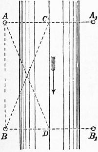
Fig. 136.

Let AB (fig. 136) be a measured base line strictly parallel to the thread of the stream, and AA1, BB1 lines at right angles to AB marked out by ranging rods at A1 and B1. Suppose observers stationed at A and B with sextants or theodolites, and let CD be the path of any float down stream. As the float approaches AA1, the observer at B keeps it on the cross wire of his instrument. The observer at A observes the instant of the float reaching the line AA1, and signals to B who then reads off the angle ABC. Similarly, as the float approaches BB1, the observer at A keeps it in sight, and when signalled to by B reads the angle BAD. The data so obtained are sufficient for plotting the path of the float and determining the distances AC, BD.