VOLUME XI SLICE VI Geodesy to Geometry (continued 13)

40. The tangents at a point of a surface which bisect the angles between the chief tangents are called the principal tangents at the point. They are at right angles, and together with the normal constitute a convenient set of rectangular axes to which to refer the surface when its properties near the point are under discussion. At a special point which is such that the chief tangents there run to the circular points at infinity in the tangent plane, the principal tangents are indeterminate; such a special point is called an umbilic of the surface.

There are two singly infinite systems of curves on a surface, a pair cutting one another at right angles through every point upon it, all tangents to which are principal tangents of the surface at their respective points of contact. These are called lines of curvature, because of a property next to be mentioned.

As a point Q moves in an arbitrary direction on a surface from coincidence with a chosen point P, the normal at it, as a rule, at once fails to meet the normal at P; but, if it takes the direction of a line of curvature through P, this is instantaneously not the case. We have thus on the normal two centres of curvature, and the distances of these from the point on the surface are the two principal radii of curvature of the surface at that point; these are also the radii of curvature of the sections of the surface by planes through the normal and the two principal tangents respectively; or say they are the radii of curvature of the normal sections through the two principal tangents respectively. Take at the point the axis of z in the direction of the normal, and those of x and y in the directions of the principal tangents respectively, then, if the radii of curvature be a, b (the signs being such that the coordinates of the two centres of curvature are z = a and z = b respectively), the surface has in the neighbourhood of the point the form of the paraboloid

z = x² + y² ,

2a 2b

and the chief-tangents are determined by the equation 0 = x²/2a + y²/2b. The two centres of curvature may be on the same side of the point or on opposite sides; in the former case a and b have the same sign, the paraboloid is elliptic, and the chief-tangents are imaginary; in the latter case a and b have opposite signs, the paraboloid is hyperbolic, and the chief-tangents are real.

The normal sections of the surface and the paraboloid by the same plane have the same radius of curvature; and it thence readily follows that the radius of curvature of a normal section of the surface by a plane inclined at an angle θ to that of zx is given by the equation

1 = cos² θ + sin² θ .

ρ a b

The section in question is that by a plane through the normal and a line in the tangent plane inclined at an angle θ to the principal tangent along the axis of x. To complete the theory, consider the section by a plane having the same trace upon the tangent plane, but inclined to the normal at an angle φ; then it is shown without difficulty (Meunier’s theorem) that the radius of curvature of this inclined section of the surface is = ρ cos φ.

Authorities.—The above article is largely based on that by Arthur Cayley in the 9th edition of this work. Of early and important recent publications on analytical geometry, special mention is to be made of R. Descartes, Géométrie (Leyden, 1637); John Wallis, Tractatus de sectionibus conicis nova methodo expositis (1655, Opera mathematica, i., Oxford, 1695); de l’Hospital, Traité analytique des sections coniques (Paris, 1720); Leonhard Euler, Introductio in analysin infinitorum, ii. (Lausanne, 1748); Gaspard Monge, “Application d’algèbre à la géométrie” (Journ. École Polytech., 1801); Julius Plücker, Analytisch-geometrische Entwickelungen, 3 Bde. (Essen, 1828-1831); System der analytischen Geometrie (Berlin, 1835); G. Salmon, A Treatise on Conic Sections (Dublin, 1848; 6th ed., London, 1879); Ch. Briot and J. Bouquet, Leçons de géométrie analytique (Paris, 1851; 16th ed., 1897); M. Chasles, Traité de géométrie supérieure (Paris, 1852); Wilhelm Fiedler, Analytische Geometrie der Kegelschnitte nach G. Salmon frei bearbeitet (Leipzig, 5te Aufl., 1887-1888); N.M. Ferrers, An Elementary Treatise on Trilinear Coordinates (London, 1861); Otto Hesse, Vorlesungen aus der analytischen Geometrie (Leipzig, 1865, 1881); W.A. Whitworth, Trilinear Coordinates and other Methods of Modern Analytical Geometry (Cambridge, 1866); J. Booth, A Treatise on Some New Geometrical Methods (London, i., 1873; ii., 1877); A. Clebsch-F. Lindemann, Vorlesungen über Geometrie, Bd. i. (Leipzig, 1876, 2te Aufl., 1891); R. Baltser, Analytische Geometrie (Leipzig, 1882); Charlotte A. Scott, Modern Methods of Analytical Geometry (London, 1894); G. Salmon, A Treatise on the Analytical Geometry of three Dimensions (Dublin, 1862; 4th ed., 1882); Salmon-Fiedler, Analytische Geometrie des Raumes (Leipzig, 1863; 4te Aufl., 1898); P. Frost, Solid Geometry (London, 3rd ed., 1886; 1st ed., Frost and J. Wolstenholme). See also E. Pascal, Repertorio di matematiche superiori, II. Geometria (Milan, 1900), and articles now appearing in the Encyklopädie der mathematischen Wissenschaften, Bd. iii. 1, 2.

(E. B. El.)

V. Line Geometry

Line geometry is the name applied to those geometrical investigations in which the straight line replaces the point as element. Just as ordinary geometry deals primarily with points and systems of points, this theory deals in the first instance with straight lines and systems of straight lines. In two dimensions there is no necessity for a special line geometry, inasmuch as the straight line and the point are interchangeable by the principle of duality; but in three dimensions the straight line is its own reciprocal, and for the better discussion of systems of lines we require some new apparatus, e.g., a system of coordinates applicable to straight lines rather than to points. The essential features of the subject are most easily elucidated by analytical methods: we shall therefore begin with the notion of line coordinates, and in order to emphasize the merits of the system of coordinates ultimately adopted, we first notice a system without these advantages, but often useful in special investigations.

In ordinary Cartesian coordinates the two equations of a straight line may be reduced to the form y = rx + s, z = tx + u, and r, s, t, u may be regarded as the four coordinates of the line. These coordinates lack symmetry: moreover, in changing from one base of reference to another the transformation is not linear, so that the degree of an equation is deprived of real significance. For purposes of the general theory we employ homogeneous coordinates; if x1y1z1w1 and x2y2z2w2 are two points on the line, it is easily verified that the six determinants of the array

x1y1z1w1

x2y2z2w2

are in the same ratios for all point-pairs on the line, and further, that when the point coordinates undergo a linear transformation so also do these six determinants. We therefore adopt these six determinants for the coordinates of the line, and express them by the symbols l, λ, m, μ, n, ν where l = x1w2 − x2w1, λ = y1z2 − y2z1, &c. There is the further advantage that if a1b1c1d1 and a2b2c2d2 be two planes through the line, the six determinants

a1b1c1d1

a2b2c2d2

are in the same ratios as the foregoing, so that except as regards a factor of proportionality we have λ = b1c2 − b2c1, l = c1d2 − c2d1, &c. The identical relation lλ + mμ + nν = o reduces the number of independent constants in the six coordinates to four, for we are only concerned with their mutual ratios; and the quadratic character of this relation marks an essential difference between point geometry and line geometry. The condition of intersection of two lines is

lλ′ + l′λ + mμ′ + m′μ + nν′ + n′ν = 0

where the accented letters refer to the second line. If the coordinates are Cartesian and l, m, n are direction cosines, the quantity on the left is the mutual moment of the two lines.

Since a line depends on four constants, there are three distinct types of configurations arising in line geometry—those containing a triply-infinite, a doubly-infinite and a singly-infinite number of lines; they are called Complexes, Congruences, and Ruled Surfaces or Skews respectively. A Complex is thus a system of lines satisfying one condition—that is, the coordinates are connected by a single relation; and the degree of the complex is the degree of this equation supposing it to be algebraic. The lines of a complex of the nth degree which pass through any point lie on a cone of the nth degree, those which lie in any plane envelop a curve of the nth class and there are n lines of the complex in any plane pencil; the last statement combines the former two, for it shows that the cone is of the nth degree and the curve is of the nth class. To find the lines common to four complexes of degrees n1, n2, n3, n4, we have to solve five equations, viz. the four complex equations together with the quadratic equation connecting the line coordinates, therefore the number of common lines is 2n1n2n3n4. As an example of complexes we have the lines meeting a twisted curve of the nth degree, which form a complex of the nth degree.

A Congruence is the set of lines satisfying two conditions: thus a finite number m of the lines pass through any point, and a finite number n lie in any plane; these numbers are called the degree and class respectively, and the congruence is symbolically written (m, n).

The simplest example of a congruence is the system of lines constituted by all those that pass through m points and those that lie in n planes; through any other point there pass m of these lines, and in any other plane there lie n, therefore the congruence is of degree m and class n. It has been shown by G.H. Halphen that the number of lines common to two congruences is mm′ + nn′, which may be verified by taking one of them to be of this simple type. The lines meeting two fixed lines form the general (1, 1) congruence; and the chords of a twisted cubic form the general type of a (1, 3) congruence; Halphen’s result shows that two twisted cubics have in general ten common chords. As regards the analytical treatment, the difficulty is of the same nature as that arising in the theory of curves in space, for a congruence is not in general the complete intersection of two complexes.

A Ruled Surface, Regulus or Skew is a configuration of lines which satisfy three conditions, and therefore depend on only one parameter. Such lines all lie on a surface, for we cannot draw one through an arbitrary point; only one line passes through a point of the surface; the simplest example, that of a quadric surface, is really two skews on the same surface.

The degree of a ruled surface qua line geometry is the number of its generating lines contained in a linear complex. Now the number which meets a given line is the degree of the surface qua point geometry, and as the lines meeting a given line form a particular case of linear complex, it follows that the degree is the same from whichever point of view we regard it. The lines common to three complexes of degrees, n1n2n3, form a ruled surface of degree 2n1n2n3; but not every ruled surface is the complete intersection of three complexes.

In the case of a complex of the first degree (or linear complex) the lines through a fixed point lie in a plane called the polar plane or nul-plane of that point, and those lying in a fixed plane pass through a point called the nul-point or pole of the Linear complex. plane. If the nul-plane of A pass through B, then the nul-plane of B will pass through A; the nul-planes of all points on one line l1 pass through another line l2. The relation between l1 and l2 is reciprocal; any line of the complex that meets one will also meet the other, and every line meeting both belongs to the complex. They are called conjugate or polar lines with respect to the complex. On these principles can be founded a theory of reciprocation with respect to a linear complex.

This may be aptly illustrated by an elegant example due to A. Voss. Since a twisted cubic can be made to satisfy twelve conditions, it might be supposed that a finite number could be drawn to touch four given lines, but this is not the case. For, suppose one such can be drawn, then its reciprocal with respect to any linear complex containing the four lines is a curve of the third class, i.e. another twisted cubic, touching the same four lines, which are unaltered in the process of reciprocation; as there is an infinite number of complexes containing the four lines, there is an infinite number of cubics touching the four lines, and the problem is poristic.

The following are some geometrical constructions relating to the unique linear complex that can be drawn to contain five arbitrary lines:

To construct the nul-plane of any point O, we observe that the two lines which meet any four of the given five are conjugate lines of the complex, and the line drawn through O to meet them is therefore a ray of the complex; similarly, by choosing another four we can find another ray through O: these rays lie in the nul-plane, and there is clearly a result involved that the five lines so obtained all lie in one plane. A reciprocal construction will enable us to find the nul-point of any plane. Proceeding now to the metrical properties and the statical and dynamical applications, we remark that there is just one line such that the nul-plane of any point on it is perpendicular to it. This is called the central axis; if d be the shortest distance, θ the angle between it and a ray of the complex, then d tan θ = p, where p is a constant called the pitch or parameter. Any system of forces can be reduced to a force R along a certain line, and a couple G perpendicular to that line; the lines of nul-moment for the system form a linear complex of which the given line is the central axis and the quotient G/R is the pitch. Any motion of a rigid body can be reduced to a screw motion about a certain line, i.e. to an angular velocity ω about that line combined with a linear velocity u along the line. The plane drawn through any point perpendicular to the direction of its motion is its nul-plane with respect to a linear complex having this line for central axis, and the quotient u/ω for pitch (cf. Sir R.S. Ball, Theory of Screws).

The following are some properties of a configuration of two linear complexes:

The lines common to the two-complexes also belong to an infinite number of linear complexes, of which two reduce to single straight lines. These two lines are conjugate lines with respect to each of the complexes, but they may coincide, and then some simple modifications are required. The locus of the central axis of this system of complexes is a surface of the third degree called the cylindroid, which plays a leading part in the theory of screws as developed synthetically by Ball. Since a linear complex has an invariant of the second degree in its coefficients, it follows that two linear complexes have a lineo-linear invariant. This invariant is fundamental: if the complexes be both straight lines, its vanishing is the condition of their intersection as given above; if only one of them be a straight line, its vanishing is the condition that this line should belong to the other complex. When it vanishes for any two complexes they are said to be in involution or apolar; the nul-points P, Q of any plane then divide harmonically the points in which the plane meets the common conjugate lines, and each complex is its own reciprocal with respect to the other. As regards a configuration of these linear complexes, the common lines from one system of generators of a quadric, and the doubly infinite system of complexes containing the common lines, include an infinite number of straight lines which form the other system of generators of the same quadric.

If the equation of a linear complex is Al + Bm + Cn + Dλ + Eμ + Fν = 0, then for a line not belonging to the complex we may regard the expression on the left-hand side as a multiple of the moment of the line with respect to the complex, the word General line coordinates. moment being used in the statical sense; and we infer that when the coordinates are replaced by linear functions of themselves the new coordinates are multiples of the moments of the line with respect to six fixed complexes. The essential features of this coordinate system are the same as those of the original one, viz. there are six coordinates connected by a quadratic equation, but this relation has in general a different form. By suitable choice of the six fundamental complexes, as they may be called, this connecting relation may be brought into other simple forms of which we mention two: (i.) When the six are mutually in involution it can be reduced to x1² + x2² + x3² + x4² + x5² + x6² = 0; (ii.) When the first four are in involution and the other two are the lines common to the first four it is x1² + x2² + x3² + x4² − 2x5x6 = 0. These generalized coordinates might be explained without reference to actual magnitude, just as homogeneous point coordinates can be; the essential remark is that the equation of any coordinate to zero represents a linear complex, a point of view which includes our original system, for the equation of a coordinate to zero represents all the lines meeting an edge of the fundamental tetrahedron.

The system of coordinates referred to six complexes mutually in involution was introduced by Felix Klein, and in many cases is more useful than that derived directly from point coordinates; e.g. in the discussion of quadratic complexes: by means of it Klein has developed an analogy between line geometry and the geometry of spheres as treated by G. Darboux and others. In fact, in that geometry a point is represented by five coordinates, connected by a relation of the same type as the one just mentioned when the five fundamental spheres are mutually at right angles and the equation of a sphere is of the first degree. Extending this to four dimensions of space, we obtain an exact analogue of line geometry, in which (i.) a point corresponds to a line; (ii.) a linear complex to a hypersphere; (iii.) two linear complexes in involution to two orthogonal hyperspheres; (iv.) a linear complex and two conjugate lines to a hypersphere and two inverse points. Many results may be obtained by this principle, and more still are suggested by trying to extend the properties of circles to spheres in three and four dimensions. Thus the elementary theorem, that, given four lines, the circles circumscribed to the four triangles formed by them are concurrent, may be extended to six hyperplanes in four dimensions; and then we can derive a result in line geometry by translating the inverse of this theorem. Again, just as there is an infinite number of spheres touching a surface at a given point, two of them having contact of a closer nature, so there is an infinite number of linear complexes touching a non-linear complex at a given line, and three of these have contact of a closer nature (cf. Klein, Math. Ann. v.).

Sophus Lie has pointed out a different analogy with sphere geometry. Suppose, in fact, that the equation of a sphere of radius r is

x² + y² + z² + 2ax + 2by + 2cz + d = 0,

so that r² = a² + b² + c² − d; then introducing the quantity e to make this equation homogeneous, we may regard the sphere as given by the six coordinates a, b, c, d, e, r connected by the equation a² + b² + c² − r² − de = 0, and it is easy to see that two spheres touch, if the polar form 2aa1 + 2bb1 + 2cc1 − 2rr1 − de1 − d1e vanishes. Comparing this with the equation x1² + x2² + x3² + x4² − 2x5x6 = 0 given above, it appears that this sphere geometry and line geometry are identical, for we may write a = x1, b = x2, c = x3, r = x4δ − 1, d = x5, e = ½x6; but it is to be noticed that a sphere is really replaced by two lines whose coordinates only differ in the sign of x4, so that they are polar lines with respect to the complex x4 = 0. Two spheres which touch correspond to two lines which intersect, or more accurately to two pairs of lines (p, p′) and (q, q′), of which the pairs (p, q) and (p′, q′) both intersect. By this means the problem of describing a sphere to touch four given spheres is reduced to that of drawing a pair of lines (t, t′) (of which t intersects one line of the four pairs (pp′), (qq′), (rr′), (ss′), and t′ intersects the remaining four). We may, however, ignore the accented letters in translating theorems, for a configuration of lines and its polar with respect to a linear complex have the same projective properties. In Lie’s transformation a linear complex corresponds to the totality of spheres cutting a given sphere at a given angle. A most remarkable result is that lines of curvature in the sphere geometry become asymptotic lines in the line geometry.

Some of the principles of line geometry may be brought into clearer light by admitting the ideas of space of four and five dimensions.

Thus, regarding the coordinates of a line as homogeneous coordinates in five dimensions, we may say that line geometry is equivalent to geometry on a quadric surface in five dimensions. A linear complex is represented by a hyperplane section; and if two such complexes are in involution, the corresponding hyperplanes are conjugate with respect to the fundamental quadric. By projecting this quadric stereographically into space of four dimensions we obtain Klein’s analogy. In the same way geometry in a linear complex is equivalent to geometry on a quadric in four dimensions; when two lines intersect the representative points are on the same generator of this quadric. Stereographic projection, therefore, converts a curve in a linear complex, i.e. one whose tangents all belong to the complex, into one whose tangents intersect a fixed conic: when this conic is the imaginary circle at infinity the curve is what Lie calls a minimal curve. Curves in a linear complex have been extensively studied. The osculating plane at any point of such a curve is the nul-plane of the point with respect to the complex, and points of superosculation always coincide in pairs at the points of contact of stationary tangents. When a point of such a curve is given, the osculating plane is determined, hence all the curves through a given point with the same tangent have the same torsion.

The lines through a given point that belong to a complex of the nth degree lie on a cone of the nth degree: if this cone has a double line the point is said to be a singular point. Similarly, Non-linear complexes. a plane is said to be singular when the envelope of the lines in it has a double tangent. It is very remarkable that the same surface is the locus of the singular points and the envelope of the singular planes: this surface is called the singular surface, and both its degree and class are in general 2n(n − 1)², which is equal to four for the quadratic complex.

The singular lines of a complex F = 0 are the lines common to F and the complex

δF δF + δF δF + δF δF = 0.

δl δλ δm δμ δn δν

As already mentioned, at each line l of a complex there is an infinite number of tangent linear complexes, and they all contain the lines adjacent to l. If now l be a singular line, these complexes all reduce to straight lines which form a plane pencil containing the line l. Suppose the vertex of the pencil is A, its plane a, and one of its lines ξ, then l′ being a complex line near l, meets ξ, or more accurately the mutual moment of l′, and is of the second order of small quantities. If P be a point on l, a line through P quite near l in the plane a will meet ξ and is therefore a line of the complex; hence the complex-cones of all points on l touch a and the complex-curves of all planes through l touch l at A. It follows that l is a double line of the complex-cone of A, and a double tangent of the complex-curve of a. Conversely, a double line of a cone or curve is a singular line, and a singular line clearly touches the curves of all planes through it in the same point. Suppose now that the consecutive line l′ is also a singular line, A′ being the allied singular point, a′ the singular plane and ξ′ any line of the pencil (A′, a′) so that ξ′ is a tangent line at l′ to the complex: the mutual moments of the pairs l′, ξ and l, ξ are each of the second order; hence the plane a′ meets the lines l and ξ′ in two points very near A. This being true for all singular planes, near a the point of contact of a with its envelope is in A, i.e. the locus of singular points is the same as the envelope of singular planes. Further, when a line touches a complex it touches the singular surface, for it belongs to a plane pencil like (Aa), and thus in Klein’s analogy the analogue of a focus of a hyper-surface being a bitangent line of the complex is also a bitangent line of the singular surface. The theory of cosingular complexes is thus brought into line with that of confocal surfaces in four dimensions, and guided by these principles the existence of cosingular quadratic complexes can easily be established, the analysis required being almost the same as that invented for confocal cyclides by Darboux and others. Of cosingular complexes of higher degree nothing is known.

Following J. Plücker, we give an account of the lines of a quadratic complex that meet a given line.

The cones whose vertices are on the given line all pass through eight fixed points and envelop a surface of the fourth degree; the conics whose planes contain the given line all lie on a surface of the fourth class and touch eight fixed planes. It is easy to see by elementary geometry that these two surfaces are identical. Further, the given line contains four singular points A1, A2, A3, A4, and the planes into which their cones degenerate are the eight common tangent planes mentioned above; similarly, there are four singular planes, a1, a2, a3, a4, through the line, and the eight points into which their conics degenerate are the eight common points above. The locus of the pole of the line with respect to all the conics in planes through it is a straight line called the polar line of the given one; and through this line passes the polar plane of the given line with respect to each of the cones. The name polar is applied in the ordinary analytical sense; any line has an infinite number of polar complexes with respect to the given complex, for the equation of the latter can be written in an infinite number of ways; one of these polars is a straight line, and is the polar line already introduced. The surface on which lie all the conics through a line l is called the Plücker surface of that line: from the known properties of (2, 2) correspondences it can be shown that the Plücker surface of l cuts l1 in a range of the same cross ratio as that of the range in which the Plücker surface of l1 cuts l. Applying this to the case in which l1 is the polar of l, we find that the cross ratios of (A1, A2, A3, A4) and (a1, a2, a3, a4) are equal. The identity of the locus of the A′s with the envelope of the a′s follows at once; moreover, a line meets the singular surface in four points having the same cross ratio as that of the four tangent planes drawn through the line to touch the surface. The Plücker surface has eight nodes, eight singular tangent planes, and is a double line. The relation between a line and its polar line is not a reciprocal one with respect to the complex; but W. Stahl has pointed out that the relation is reciprocal as far as the singular surface is concerned.

To facilitate the discussion of the general quadratic complex we Quadratic complexes. introduce Klein’s canonical form. We have, in fact, to deal with two quadratic equations in six variables; and by suitable linear transformations these can be reduced to the form

a1x12 + a2x22 + a3x32 + a4x42 + a5x52 + a6x62 = 0

x12 + x22 + x32 + x42 + x52 + x62 = 0

subject to certain exceptions, which will be mentioned later.

Taking the first equation to be that of the complex, we remark that both equations are unaltered by changing the sign of any coordinate; the geometrical meaning of this is, that the quadratic complex is its own reciprocal with respect to each of the six fundamental complexes, for changing the sign of a coordinate is equivalent to taking the polar of a line with respect to the corresponding fundamental complex. It is easy to establish the existence of six systems of bitangent linear complexes, for the complex l1x1 + l2x2 + l3x3 + l4x4 + l5x5 + l6x6 = 0 is a bitangent when

l1 = 0, and l2² + l3² + l4² + l5² + l6² = 0,

a2 − a1 a3 − a1 a4 − a1 a5 − a1 a6 − a1

and its lines of contact are conjugate lines with respect to the first fundamental complex. We therefore infer the existence of six systems of bitangent lines of the complex, of which the first is given by

x1 = 0, x2² + x3² + x4² + x5² + x6² = 0,

a2 − a1 a3 − a1 a4 − a1 a5 − a1 a6 − a1

Each of these lines is a bitangent of the singular surface, which is therefore completely determined as being the focal surface of the (2, 2) congruence above. It is thence easy to verify that the two complexes Σax2 = 0 and Σbx2 = 0 are cosingular if br = arλ + μ/arν + ρ.

The singular surface of the general quadratic complex is the famous quartic, with sixteen nodes and sixteen singular tangent planes, first discovered by E.E. Kümmer.

We cannot give a full account of its properties here, but we deduce at once from the above that its bitangents break up into six (2, 2) congruences, and the six linear complexes containing these are mutually in involution. The nodes of the singular surface are points whose complex cones are coincident planes, and the complex conic in a singular tangent plane consists of two coincident points. This configuration of sixteen points and planes has many interesting properties; thus each plane contains six points which lie on a conic, while through each point there pass six planes which touch a quadric cone. In many respects the Kümmer quartic plays a part in three dimensions analogous to the general quartic curve in two; it further gives a natural representation of certain relations between hyperelliptic functions (cf. R.W.H.T. Hudson, Kümmer’s Quartic, 1905).

As might be expected from the magnitude of a form in six variables, the number of projectivally distinct varieties of quadratic complexes is very great; and in fact Adolf Weiler, by whom the Classification of quadratic complexes. question was first systematically studied on lines indicated by Klein, enumerated no fewer than forty-nine different types. But the principle of the classification is so important, and withal so simple, that we give a brief sketch which indicates its essential features.

We have practically to study the intersection of two quadrics F and F′ in six variables, and to classify the different cases arising we make use of the results of Karl Weierstrass on the equivalence conditions of two pairs of quadratics. As far as at present required, they are as follows: Suppose that the factorized form of the determinantal equation Disct (F + λF′) = 0 is

(λ − α)s1 + s2 + s3 ... (λ − β)t1 + t2 + t3 + ... ...

where the root α occurs s1 + s2 + s3 ... times in the determinant, s2 + s3 ... times in every first minor, s3 + ... times in every second minor, and so on; the meaning of each exponent is then perfectly definite. Every factor of the type (λ − α)s is called an elementartheil (elementary divisor) of the determinant, and the condition of equivalence of two pairs of quadratics is simply that their determinants have the same elementary divisors. We write the pair of forms symbolically thus [(s1s2 ...), (t1t2 ...), ...], letters in the inner brackets referring to the same factor. Returning now to the two quadratics representing the complex, the sum of the exponents will be six, and two complexes are put in the same class if they have the same symbolical expression; i.e. the actual values of the roots of the determinantal equation need not be the same for both, but their manner of occurrence, as far as here indicated, must be identical in the two. The enumeration of all possible cases is thus reduced to a simple question in combinatorial analysis, and the actual study of any particular case is much facilitated by a useful rule of Klein’s for writing down in a simple form two quadratics belonging to a given class—one of which, of course, represents the equation connecting line coordinates, and the other the equation of the complex. The general complex is naturally [111111]; the complex of tangents to a quadric is [(111), (111)] and that of lines meeting a conic is [(222)]. Full information will be found in Weiler’s memoir, Math. Ann. vol. vii.

The detailed study of each variety of complex opens up a vast subject; we only mention two special cases, the harmonic complex and the tetrahedral complex.

The harmonic complex, first studied by Battaglini, is generated in an infinite number of ways by the lines cutting two quadrics harmonically. Taking the most general case, and referring the quadrics to their common self-conjugate tetrahedron, we can find its equation in a simple form, and verify that this complex really depends only on seventeen constants, so that it is not the most general quadratic complex. It belongs to the general type in so far as it is discussed above, but the roots of the determinant are in involution. The singular surface is the “tetrahedroid” discussed by Cayley. As a particular case, from a metrical point of view, we have L.F. Painvin’s complex generated by the lines of intersection of perpendicular tangent planes of a quadric, the singular surface now being Fresnel’s wave surface. The tetrahedral or Reye complex is the simplest and best known of proper quadratic complexes. It is generated by the lines which cut the faces of a tetrahedron in a constant cross ratio, and therefore by those subtending the same cross ratio at the four vertices. The singular surface is made up of the faces or the vertices of the fundamental tetrahedron, and each edge of this tetrahedron is a double line of the complex. The complex was first discussed by K.T. Reye as the assemblage of lines joining corresponding points in a homographic transformation of space, and this point of view leads to many important and elegant properties. A (metrically) particular case of great interest is the complex generated by the normals to a family of confocal quadrics, and for many investigations it is convenient to deal with this complex referred to the principal axes. For example, Lie has developed the theory of curves in a Reye complex (i.e. curves whose tangents belong to the complex) as solutions of a differential equation of the form (b − c)xdydz + (c − a)ydzdx + (a − b)zdxdy = 0, and we can simplify this equation by a logarithmic transformation. Many theorems connecting complexes with differential equations have been given by Lie and his school. A line complex, in fact, corresponds to a Mongian equation having ∞3 line integrals.

As the coordinates of a line belonging to a congruence are functions of two independent parameters, the theory of congruences is analogous to that of surfaces, and we may regard it as a fundamental inquiry to find the simplest form of surface into which Congruences. a given congruence can be transformed. Most of those whose properties have been extensively discussed can be represented on a plane by a birational transformation. But in addition to the difficulties of the theory of algebraic surfaces, a subject still in its infancy, the theory of congruences has other difficulties in that a congruence is seldom completely represented, even by two equations.

A fundamental theorem is that the lines of a congruence are in general bitangents of a surface; in fact, since the condition of intersection of two consecutive straight lines is ldλ + dmdμ + dndν = 0, a line l of the congruence meets two adjacent lines, say l1 and l2. Suppose l, l1 lie in the plane pencil (A1a1) and l, l2 in the plane pencil (A2a2), then the locus of the A′s is the same as the envelope of the a′s, but a2 is the tangent plane at A1 and a1 at A2. This surface is called the focal surface of the congruence, and to it all the lines l are bitangent. The distinctive property of the points A is that two of the congruence lines through them coincide, and in like manner the planes a each contain two coincident lines. The focal surface consists of two sheets, but one or both may degenerate into curves; thus, for example, the normals to a surface are bitangents of the surface of centres, and in the case of Dupin’s cyclide this surface degenerates into two conics.

In the discussion of congruences it soon becomes necessary to introduce another number r, called the rank, which expresses the number of plane pencils each of which contains an arbitrary line and two lines of the congruence. The order of the focal surface is 2m(n − 1) − 2r, and its class is m(m − 1) − 2r. Our knowledge of congruences is almost exclusively confined to those in which either m or n does not exceed two. We give a brief account of those of the second order without singular lines, those of order unity not being especially interesting. A congruence generally has singular points through which an infinite number of lines pass; a singular point is said to be of order r when the lines through it lie on a cone of the rth degree. By means of formulae connecting the number of singular points and their orders with the class m of quadratic congruence Kümmer proved that the class cannot exceed seven. The focal surface is of degree four and class 2m; this kind of quartic surface has been extensively studied by Kümmer, Cayley, Rohn and others. The varieties (2, 2), (2, 3), (2, 4), (2, 5) all belong to at least one Reye complex; and so also does the most important class of (2, 6) congruences which includes all the above as special cases. The congruence (2, 2) belongs to a linear complex and forty different Reye complexes; as above remarked, the singular surface is Kümmer’s sixteen-nodal quartic, and the same surface is focal for six different congruences of this variety. The theory of (2, 2) congruences is completely analogous to that of the surfaces called cyclides in three dimensions. Further particulars regarding quadratic congruences will be found in Kümmer’s memoir of 1866, and the second volume of Sturm’s treatise. The properties of quadratic congruences having singular lines, i.e. degenerate focal surfaces, are not so interesting as those of the above class; they have been discussed by Kümmer, Sturm and others.

Since a ruled surface contains only ∞¹ elements, this theory is practically the same as that of curves. If a linear complex contains more than n generators of a ruled surface of the nth degree, it contains all the generators, hence for n = 2 there are Ruled surfaces. three linearly independent complexes, containing all the generators, and this is a well-known property of quadric surfaces. In ruled cubics the generators all meet two lines which may or may not coincide; these two cases correspond to the two main classes of cubics discussed by Cayley and Cremona. As regards ruled quartics, the generators must lie in one and may lie in two linear complexes. The first class is equivalent to a quartic in four dimensions and is always rational, but the latter class has to be subdivided into the elliptic and the rational, just like twisted quartic curves. A quintic skew may not lie in a linear complex, and then it is unicursal, while of sextics we have two classes not in a linear complex, viz. the elliptic variety, having thirty-six places where a linear complex contains six consecutive generators, and the rational, having six such places.

The general theory of skews in two linear complexes is identical with that of curves on a quadric in three dimensions and is known. But for skews lying in only one linear complex there are difficulties; the curve now lies in four dimensions, and we represent it in three by stereographic projection as a curve meeting a given plane in n points on a conic. To find the maximum deficiency for a given degree would probably be difficult, but as far as degree eight the space-curve theory of Halphen and Nöther can be translated into line geometry at once. When the skew does not lie in a linear complex at all the theory is more difficult still, and the general theory clearly cannot advance until further progress is made in the study of twisted curves.

References.—The earliest works of a general nature are Plücker, Neue Geometrie des Raumes (Leipzig, 1868); and Kümmer, “Über die algebraischen Strahlensysteme,” Berlin Academy (1866). Systematic development on purely synthetic lines will be found in the three volumes of Sturm, Liniengeometrie (Leipzig, 1892, 1893, 1896); vol. i. deals with the linear and Reye complexes, vols. ii. and iii. with quadratic congruences and complexes respectively. For a highly suggestive review by Gino Loria see Bulletin des sciences mathématiques (1893, 1897). A shorter treatise, giving a very interesting account of Klein’s coordinates, is the work of Koenigs, La Géométrie réglée et ses applications (Paris, 1898). English treatises are C.M. Jessop, Treatise on the Line Complex (1903); R.W.H.T. Hudson, Kümmer’s Quartic (1905). Many references to memoirs on line geometry will be found in Hagen, Synopsis der höheren Mathematik, ii. (Berlin, 1894); Loria, Il passato ed il presente delle principali teorie geometriche (Milan, 1897); a clear résumé of the principal results is contained in the very elegant volume of Pascal, Repertorio di mathematiche superiori, ii. (Milan, 1900). Another treatise dealing extensively with line geometry is Lie, Geometrie der Berührungstransformationen (Leipzig, 1896). Many memoirs on the subject have appeared in the Mathematische Annalen; a full list of these will be found in the index to the first fifty volumes, p. 115. Perhaps the two memoirs which have left most impression on the subsequent development of the subject are Klein, “Zur Theorie der Liniencomplexe des ersten und zweiten Grades,” Math. Ann. ii.; and Lie, “Über Complexe, insbesondere Linien- und Kugelcomplexe,” Math. Ann. v.

(J. H. Gr.)

VI. Non-Euclidean Geometry

The various metrical geometries are concerned with the properties of the various types of congruence-groups, which are defined in the study of the axioms of geometry and of their immediate consequences. But this point of view of the subject is the outcome of recent research, and historically the subject has a different origin. Non-Euclidean geometry arose from the discussion, extending from the Greek period to the present day, of the various assumptions which are implicit in the traditional Euclidean system of geometry. In the course of these investigations it became evident that metrical geometries, each internally consistent but inconsistent in many respects with each other and with the Euclidean system, could be developed. A short historical sketch will explain this origin of the subject, and describe the famous and interesting progress of thought on the subject. But previously a description of the chief characteristic properties of elliptic and of hyperbolic geometries will be given, assuming the standpoint arrived at below under VII. Axioms of Geometry.

First assume the equation to the absolute (cf. loc. cit.) to be w² − x² − y² − z² = 0. The absolute is then real, and the geometry is hyberbolic.

The distance (d12) between the two points (x1, y1, z1, w1) and (x2, y2, z2, w2) is given by

cosh (d12/γ) = (w1w2 − x1x2 − y1y2 − z1z2) / {(w1² − x1² − y1² − z1²) (w2² − x2² − y2² − z2²)}1/2

(1)

The only points to which the metrical geometry applies are those within the region enclosed by the quadric; the other points are “improper ideal points.” The angle (θ12) between two planes, l1x + m1y + n1z + r1w = 0 and l2x + m2y + n2z + r2w = 0, is given by

cos θ12 = (l1l2 + m1m2 + n1n2 − r1r2) / {(l1² + m1² + n1² − r1²) (l2² + m2² + n2² − r2²)}1/2

(2)

These planes only have a real angle of inclination if they possess a line of intersection within the actual space, i.e. if they intersect. Planes which do not intersect possess a shortest distance along a line which is perpendicular to both of them. If this shortest distance is δ12, we have

cosh (δ12/γ) = (l1l2 + m1m2 + n1n2 − r1r2) / {(l1² + m1² + n1² − r1²) (l2² + m2² + n2² − r2²)}1/2

(3)

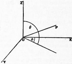
Fig. 67.

Thus in the case of the two planes one and only one of the two, θ12 and δ12, is real. The same considerations hold for coplanar straight lines (see VII. Axioms of Geometry). Let O (fig. 67) be the point (0, 0, 0, 1), OX the line y = 0, z = 0, OY the line z = 0, x = 0, and OZ the line x = 0, y = 0. These are the coordinate axes and are at right angles to each other. Let P be any point, and let ρ be the distance OP, θ the angle POZ, and φ the angle between the planes ZOX and ZOP. Then the coordinates of P can be taken to be

sinh (ρ/γ) sin θ cos φ, sinh (ρ/γ) sin θ sin φ, sinh (ρ/γ) cos θ, cosh (ρ/γ).

If ABC is a triangle, and the sides and angles are named according to the usual convention, we have

sinh (a/γ) / sin A = sinh (b/γ) / sin B = sinh (c/γ) / sin C,

(4)

and also

cosh (a/γ) = cosh (b/γ) cosh (c/γ) − sinh (b/γ) sinh (c/γ) cos A,

(5)

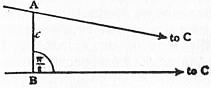
Fig. 68.

with two similar equations. The sum of the three angles of a triangle is always less than two right angles. The area of the triangle ABC is λ²(π − A − B − C). If the base BC of a triangle is kept fixed and the vertex A moves in the fixed plane ABC so that the area ABC is constant, then the locus of A is a line of equal distance from BC. This locus is not a straight line. The whole theory of similarity is inapplicable; two triangles are either congruent, or their angles are not equal two by two. Thus the elements of a triangle are determined when its three angles are given. By keeping A and B and the line BC fixed, but by making C move off to infinity along BC, the lines BC and AC become parallel, and the sides a and b become infinite. Hence from equation (5) above, it follows that two parallel lines (cf. Section VII. Axioms of Geometry) must be considered as making a zero angle with each other. Also if B be a right angle, from the equation (5), remembering that, in the limit,

cosh (a/γ) / cosh (b/γ) = cosh (a/γ) / sinh (b/γ) = 1,

we have

cos A = tanh (c/2γ)

(6).

The angle A is called by N.I. Lobatchewsky the “angle of parallelism.”

The whole theory of lines and planes at right angles to each other is simply the theory of conjugate elements with respect to the absolute, where ideal lines and planes are introduced.

Thus if l and l′ be any two conjugate lines with respect to the absolute (of which one of the two must be improper, say l′), then any plane through l′ and containing proper points is perpendicular to l. Also if p is any plane containing proper points, and P is its pole, which is necessarily improper, then the lines through P are the normals to P. The equation of the sphere, centre (x1, y1, z1, w1) and radius ρ, is

(w1² − x1² − y1² − z1²) (w² − x² − y² − z²) cosh² (ρ/γ) = (w1w − x1x − y1y − z1z)²

(7).

The equation of the surface of equal distance (σ) from the plane lx + my + nz + rw = 0 is

(l² + m² + n² − r²) (w² − x² − y² − z²) sinh² (σ/γ) = (rw + lx + my + nz)²

(8).

A surface of equal distance is a sphere whose centre is improper; and both types of surface are included in the family

k² (w² − x² − y² − z²) = (ax + by + cz + dw)²

(9).

But this family also includes a third type of surfaces, which can be looked on either as the limits of spheres whose centres have approached the absolute, or as the limits of surfaces of equal distance whose central planes have approached a position tangential to the absolute. These surfaces are called limit-surfaces. Thus (9) denotes a limit-surface, if d² − a² − b² − c² = 0. Two limit-surfaces only differ in position. Thus the two limit-surfaces which touch the plane YOZ at O, but have their concavities turned in opposite directions, have as their equations

w² − x² − y² − z² = (w ± x)².

The geodesic geometry of a sphere is elliptic, that of a surface of equal distance is hyperbolic, and that of a limit-surface is parabolic (i.e. Euclidean). The equation of the surface (cylinder) of equal distance (δ) from the line OX is

(w² − x²) tanh² (δ/γ) − y² − z² = 0.

This is not a ruled surface. Hence in this geometry it is not possible for two straight lines to be at a constant distance from each other.

Secondly, let the equation of the absolute be x² + y² + z² + w² = 0. The absolute is now imaginary and the geometry is elliptic.

The distance (d12) between the two points (x1, y1, z1, w1) and (x2, y2, z2, w2) is given by

cos (d12/γ) = ± (x1x2 + y1y2 + z1z2 + w1w2) / {(x1² + y1² + z1² + w1²) (x2² + y2² + z2² + w2²)}1/2

(10).

Thus there are two distances between the points, and if one is d12, the other is πγ-d12. Every straight line returns into itself, forming a closed series. Thus there are two segments between any two points, together forming the whole line which contains them; one distance is associated with one segment, and the other distance with the other segment. The complete length of every straight line is πγ.

The angle between the two planes l1x + m1y + n1z + r + 1w = 0 and l2x + m2y + n2z + r2w = 0 is

cos θ12 = (l1l2 + m1m2 + n1n2 + r1r2) / {(l1² + m1² + n1² +r1²) (l2² + m2² + n2² + r2²)}1/2

(11).

The polar plane with respect to the absolute of the point (x1, y1, z1, w1) is the real plane x1x + y1y + z1z + w1w = 0, and the pole of the plane l1x + m1y + n1z + r1w = 0 is the point (l1, m1, n1, r1). Thus (from equations 10 and 11) it follows that the angle between the polar planes of the points (x1, ...) and (x2, ...) is d12/γ, and that the distance between the poles of the planes (l1, ...) and (l2, ...) is γθ12. Thus there is complete reciprocity between points and planes in respect to all properties. This complete reign of the principle of duality is one of the great beauties of this geometry. The theory of lines and planes at right angles is simply the theory of conjugate elements with respect to the absolute. A tetrahedron self-conjugate with respect to the absolute has all its intersecting elements (edges and planes) at right angles. If l and l′ are two conjugate lines, the planes through one are the planes perpendicular to the other. If P is the pole of the plane p, the lines through P are the normals to the plane p. The distance from P to p is ½πγ. Thus every sphere is also a surface of equal distance from the polar of its centre, and conversely. A plane does not divide space; for the line joining any two points P and Q only cuts the plane once, in L say, then it is always possible to go from P to Q by the segment of the line PQ which does not contain L. But P and Q may be said to be separated by a plane p, if the point in which PQ cuts p lies on the shortest segment between P and Q. With this sense of “separation,” it is possible2 to find three points P, Q, R such that P and Q are separated by the plane p, but P and R are not separated by p, nor are Q and R.

Let A, B, C be any three non-collinear points, then four triangles are defined by these points. Thus if a, b, c and A, B, C are the elements of any one triangle, then the four triangles have as their elements:

(1) a, b, c, A, B, C.

(2) a, πγ − b, πγ − c, A, π − B, π − C.

(3) πγ − a, b, πγ − c, π − A, B, π − C.

(4) πγ − a, πγ − b, c, π − A, π − B, C.

The formulae connecting the elements are

sin A/sin (a/γ) = sin B/sin (b/γ) = sin C/sin (c/γ),

(12)

and

cos (a/γ) = cos (b/γ) cos (c/γ) + sin (b/γ) sin (c/γ) cos A,

(13)

with two similar equations.

Two cases arise, namely (I.) according as one of the four triangles has as its sides the shortest segments between the angular points, or (II.) according as this is not the case. When case I. holds there is said to be a “principal triangle.”3 If all the figures considered lie within a sphere of radius ¼πγ only case I. can hold, and the principal triangle is the triangle wholly within this sphere, also the peculiarities in respect to the separation of points by a plane cannot then arise. The sum of the three angles of a triangle ABC is always greater than two right angles, and the area of the triangle is γ²(A + B + C − π). Thus as in hyperbolic geometry the theory of similarity does not hold, and the elements of a triangle are determined when its three angles are given. The coordinates of a point can be written in the form

sin (ρ/γ) sin Φ cos φ, sin (ρ/γ) sin Φ sin φ, sin (ρ/γ) cos Φ, cos (ρ/γ),

where ρ, Φ and φ have the same meanings as in the corresponding formulae in hyperbolic geometry. Again, suppose a watch is laid on the plane OXY, face upwards with its centre at O, and the line 12 to 6 (as marked on dial) along the line YOY. Let the watch be continually pushed along the plane along the line OX, that is, in the direction 9 to 3. Then the line XOX being of finite length, the watch will return to O, but at its first return it will be found to be face downwards on the other side of the plane, with the line 12 to 6 reversed in direction along the line YOY. This peculiarity was first pointed out by Felix Klein. The theory of parallels as it exists in hyperbolic space has no application in elliptic geometry. But another property of Euclidean parallel lines holds in elliptic geometry, and by the use of it parallel lines are defined. For the equation of the surface (cylinder) of equal distance (δ) from the line XOX is

(x² + w²) tan² (δ/γ) − (y² + z²) = 0.

This is also the surface of equal distance, ½πγ-δ, from the line conjugate to XOX. Now from the form of the above equation this is a ruled surface, and through every point of it two generators pass. But these generators are lines of equal distance from XOX. Thus throughout every point of space two lines can be drawn which are lines of equal distance from a given line l. This property was discovered by W.K. Clifford. The two lines are called Clifford’s right and left parallels to l through the point. This property of parallelism is reciprocal, so that if m is a left parallel to l, then l is a left parallel to m. Note also that two parallel lines l and m are not coplanar. Many of those properties of Euclidean parallels, which do not hold for Lobatchewsky’s parallels in hyperbolic geometry, do hold for Clifford’s parallels in elliptic geometry. The geodesic geometry of spheres is elliptic, the geodesic geometry of surfaces of equal distance from lines (cylinders) is Euclidean, and surfaces of revolution can be found4 of which the geodesic geometry is hyperbolic. But it is to be noticed that the connectivity of these surfaces is different to that of a Euclidean plane. For instance there are only ∞² congruence transformations of the cylindrical surfaces of equal distance into themselves, instead of the ∞³ for the ordinary plane. It would obviously be possible to state “axioms” which these geodesics satisfy, and thus to define independently, and not as loci, quasi-spaces of these peculiar types. The existence of such Euclidean quasi-geometries was first pointed out by Clifford.5

In both elliptic and hyperbolic geometry the spherical geometry, i.e. the relations between the angles formed by lines and planes passing through the same point, is the same as the “spherical trigonometry” in Euclidean geometry. The constant γ, which appears in the formulae both of hyperbolic and elliptic geometry, does not by its variation produce different types of geometry. There is only one type of elliptic geometry and one type of hyperbolic geometry; and the magnitude of the constant γ in each case simply depends upon the magnitude of the arbitrary unit of length in comparison with the natural unit of length which each particular instance of either geometry presents. The existence of a natural unit of length is a peculiarity common both to hyperbolic and elliptic geometries, and differentiates them from Euclidean geometry. It is the reason for the failure of the theory of similarity in them. If γ is very large, that is, if the natural unit is very large compared to the arbitrary unit, and if the lengths involved in the figures considered are not large compared to the arbitrary unit, then both the elliptic and hyperbolic geometries approximate to the Euclidean. For from formulae (4) and (5) and also from (12) and (13) we find, after retaining only the lowest powers of small quantities, as the formulae for any triangle ABC,

a / sin A = b / sin B = c / sin C,

and

a² = b² + c² − 2bc cos A,

with two similar equations. Thus the geometries of small figures are in both types Euclidean.

History.—“In pulcherrimo Geometriae corpore,” wrote Sir Henry Savile in 1621, “duo sunt naevi, duae labes nec quod sciam plures, in quibus eluendis et emaculendis cum veterum tum recentiorum ... vigilavit industria.” Theory of parallels before Gauss. These two blemishes are the theory of parallels and the theory of proportion. The “industry of the moderns,” in both respects, has given rise to important branches of mathematics, while at the same time showing that Euclid is in these respects more free from blemish than had been previously credible. It was from endeavours to improve the theory of parallels that non-Euclidean geometry arose; and though it has now acquired a far wider scope, its historical origin remains instructive and interesting. Euclid’s “axiom of parallels” appears as Postulate V. to the first book of his Elements, and is stated thus, “And that, if a straight line falling on two straight lines make the angles, internal and on the same side, less than two right angles, the two straight lines, being produced indefinitely, meet on the side on which are the angles less than two right angles.” The original Greek is καὶ ἐὰν εἰς δύο εὐθείας εὐθεῖα ἐμπίπτουσα τὰς ἐντὸς καὶ ἐπὶ τὰ αὐτὰ μέρη γωνίας δύο ὀρθῶν ἐλάσσονας ποιῇ, ἐκβαλλομένας τὰς δύο εὐθείας ἐπ᾽ ἄπειρον συμπίπτειν, ἐφ᾽ ἃ μέρη εἰσὶν αἱ τῶν δύο ὀρθῶν ἐλάσσονες.

To Euclid’s successors this axiom had signally failed to appear self-evident, and had failed equally to appear indemonstrable. Without the use of the postulate its converse is proved in Euclid’s 28th proposition, and it was hoped that by further efforts the postulate itself could be also proved. The first step consisted in the discovery of equivalent axioms. Christoph Clavius in 1574 deduced the axiom from the assumption that a line whose points are all equidistant from a straight line is itself straight. John Wallis in 1663 showed that the postulate follows from the possibility of similar triangles on different scales. Girolamo Saccheri (1733) showed that it is sufficient to have a single triangle, the sum of whose angles is two right angles. Other equivalent forms may be obtained, but none shows any essential superiority to Euclid’s. Indeed plausibility, which is chiefly aimed at, becomes a positive demerit where it conceals a real assumption.

A new method, which, though it failed to lead to the desired goal, proved in the end immensely fruitful, was invented by Saccheri, in a work entitled Euclides ab omni naevo vindicatus (Milan, 1733). If the postulate of parallels Saccheri. is involved in Euclid’s other assumptions, contradictions must emerge when it is denied while the others are maintained. This led Saccheri to attempt a reductio ad absurdum, in which he mistakenly believed himself to have succeeded. What is interesting, however, is not his fallacious conclusion, but the non-Euclidean results which he obtains in the process. Saccheri distinguishes three hypotheses (corresponding to what are now known as Euclidean or parabolic, elliptic and hyperbolic geometry), and proves that some one of the three must be universally true. His three hypotheses are thus obtained: equal perpendiculars AC, BD are drawn from a straight line AB, and CD are joined. It is shown that the angles ACD, BDC are equal. The first hypothesis is that these are both right angles; the second, that they are both obtuse; and the third, that they are both acute. Many of the results afterwards obtained by Lobatchewsky and Bolyai are here developed. Saccheri fails to be the founder of non-Euclidean geometry only because he does not perceive the possible truth of his non-Euclidean hypotheses.

Some advance is made by Johann Heinrich Lambert in his Theorie der Parallellinien (written 1766; posthumously published 1786). Though he still believed in the necessary truth of Euclidean geometry, he confessed that, in Lambert. all his attempted proofs, something remained undemonstrated. He deals with the same three hypotheses as Saccheri, showing that the second holds on a sphere, while the third would hold on a sphere of purely imaginary radius. The second hypothesis he succeeds in condemning, since, like all who preceded Bernhard Riemann, he is unable to conceive of the straight line as finite and closed. But the third hypothesis, which is the same as Lobatchewsky’s, is not even professedly refuted.6

Non-Euclidean geometry proper begins with Karl Friedrich Gauss. The advance which he made was rather philosophical than mathematical: it was he (probably) who first recognized that the postulate of parallels is possibly Three periods of non-Euclidean geometry. false, and should be empirically tested by measuring the angles of large triangles. The history of non-Euclidean geometry has been aptly divided by Felix Klein into three very distinct periods. The first—which contains only Gauss, Lobatchewsky and Bolyai—is characterized by its synthetic method and by its close relation to Euclid. The attempt at indirect proof of the disputed postulate would seem to have been the source of these three men’s discoveries; but when the postulate had been denied, they found that the results, so far from showing contradictions, were just as self-consistent as Euclid. They inferred that the postulate, if true at all, can only be proved by observations and measurements. Only one kind of non-Euclidean space is known to them, namely, that which is now called hyperbolic. The second period is analytical, and is characterized by a close relation to the theory of surfaces. It begins with Riemann’s inaugural dissertation, which regards space as a particular case of a manifold; but the characteristic standpoint of the period is chiefly emphasized by Eugenio Beltrami. The conception of measure of curvature is extended by Riemann from surfaces to spaces, and a new kind of space, finite but unbounded (corresponding to the second hypothesis of Saccheri and Lambert), is shown to be possible. As opposed to the second period, which is purely metrical, the third period is essentially projective in its method. It begins with Arthur Cayley, who showed that metrical properties are projective properties relative to a certain fundamental quadric, and that different geometries arise according as this quadric is real, imaginary or degenerate. Klein, to whom the development of Cayley’s work is due, showed further that there are two forms of Riemann’s space, called by him the elliptic and the spherical. Finally, it has been shown by Sophus Lie, that if figures are to be freely movable throughout all space in ∞6 ways, no other three-dimensional spaces than the above four are possible.

Gauss published nothing on the theory of parallels, and it was not generally known until after his death that he had interested himself in that theory from a very early date. In 1799 he announces that Euclidean geometry Gauss. would follow from the assumption that a triangle can be drawn greater than any given triangle. Though unwilling to assume this, we find him in 1804 still hoping to prove the postulate of parallels. In 1830 he announces his conviction that geometry is not an a priori science; in the following year he explains that non-Euclidean geometry is free from contradictions, and that, in this system, the angles of a triangle diminish without limit when all the sides are increased. He also gives for the circumference of a circle of radius r the formula πk(er/k − er −/k), where k is a constant depending upon the nature of the space. In 1832, in reply to the receipt of Bolyai’s Appendix, he gives an elegant proof that the amount by which the sum of the angles of a triangle falls short of two right angles is proportional to the area of the triangle. From these and a few other remarks it appears that Gauss possessed the foundations of hyperbolic geometry, which he was probably the first to regard as perhaps true. It is not known with certainty whether he influenced Lobatchewsky and Bolyai, but the evidence we possess is against such a view.7

The first to publish a non-Euclidean geometry was Nicholas Lobatchewsky, professor of mathematics in the new university of Kazañ.8 In the place of the disputed postulate he puts the following: “All straight lines which, in Lobatchewsky. a plane, radiate from a given point, can, with respect to any other straight line in the same plane, be divided into two classes, the intersecting and the non-intersecting. The boundary line of the one and the other class is called parallel to the given line.” It follows that there are two parallels to the given line through any point, each meeting the line at infinity, like a Euclidean parallel. (Hence a line has two distinct points at infinity, and not one only as in ordinary geometry.) The two parallels to a line through a point make equal acute angles with the perpendicular to the line through the point. If p be the length of the perpendicular, either of these angles is denoted by Π(p). The determination of Π(p) is the chief problem (cf. equation (6) above); it appears finally that, with a suitable choice of the unit of length,

tan ½ Π(p) = e−p.

Before obtaining this result it is shown that spherical trigonometry is unchanged, and that the normals to a circle or a sphere still pass through its centre. When the radius of the circle or sphere becomes infinite all these normals become parallel, but the circle or sphere does not become a straight line or plane. It becomes what Lobatchewsky calls a limit-line or limit-surface. The geometry on such a surface is shown to be Euclidean, limit-lines replacing Euclidean straight lines. (It is, in fact, a surface of zero measure of curvature.) By the help of these propositions Lobatchewsky obtains the above value of Π(p), and thence the solution of triangles. He points out that his formulae result from those of spherical trigonometry by substituting ia, ib, ic, for the sides a, b, c.

John Bolyai, a Hungarian, obtained results closely corresponding to those of Lobatchewsky. These he published in an appendix to a work by his father, entitled Appendix Scientiam spatii absolute veram exhibens: a veritate aut falsitate Bolyai. Axiomatis XI. Euclidei (a priori haud unquam decidenda) independentem: adjecta ad casum falsitatis, quadratura circuli geometrica.9 This work was published in 1831, but its conception dates from 1823. It reveals a profounder appreciation of the importance of the new ideas, but otherwise differs little from Lobatchewsky’s. Both men point out that Euclidean geometry as a limiting case of their own more general system, that the geometry of very small spaces is always approximately Euclidean, that no a priori grounds exist for a decision, and that observation can only give an approximate answer. Bolyai gives also, as his title indicates, a geometrical construction, in hyperbolic space, for the quadrature of the circle, and shows that the area of the greatest possible triangle, which has all its sides parallel and all its angles zero, is πι², where i is what we should now call the space-constant.

The works of Lobatchewsky and Bolyai, though known and valued by Gauss, remained obscure and ineffective until, in 1866, they were translated into French by J. Hoüel. But Riemann. at this time Riemann’s dissertation, Über die Hypothesen, welche der Geometrie zu Grunde liegen,10 was already about to be published. In this work Riemann, without any knowledge of his predecessors in the same field, inaugurated a far more profound discussion, based on a far more general standpoint; and by its publication in 1867 the attention of mathematicians and philosophers was at last secured. (The dissertation dates from 1854, but owing to changes which Riemann wished to make in it, it remained unpublished until after his death.)

Riemann’s work contains two fundamental conceptions, that of a manifold and that of the measure of curvature of a continuous manifold possessed of what he calls flatness in the smallest parts. By means of these conceptions space is made to appear Definition of a manifold. at the end of a gradual series of more and more specialized conceptions. Conceptions of magnitude, he explains, are only possible where we have a general conception capable of determination in various ways. The manifold consists of all these various determinations, each of which is an element of the manifold. The passage from one element to another may be discrete or continuous; the manifold is called discrete or continuous accordingly. Where it is discrete two portions of it can be compared, as to magnitude, by counting; where continuous, by measurement. But measurement demands superposition, and consequently some magnitude independent of its place in the manifold. In passing, in a continuous manifold, from one element to another in a determinate way, we pass through a series of intermediate terms, which form a one-dimensional manifold. If this whole manifold be similarly caused to pass over into another, each of its elements passes through a one-dimensional manifold, and thus on the whole a two-dimensional manifold is generated. In this way we can proceed to n dimensions. Conversely, a manifold of n dimensions can be analysed into one of one dimension and one of (n − 1) dimensions. By repetitions of this process the position of an element may be at last determined by n magnitudes. We may here stop to observe that the above conception of a manifold is akin to that due to Hermann Grassmann in the first edition (1847) of his Ausdehnungslehre.11

Both concepts have been elaborated and superseded by the modern procedure in respect to the axioms of geometry, and by the conception of abstract geometry involved therein. Riemann proceeds to specialize the manifold by considerations Measure of curvature. as to measurement. If measurement is to be possible, some magnitude, we saw, must be independent of position; let us consider manifolds in which lengths of lines are such magnitudes, so that every line is measurable by every other. The coordinates of a point being x1, x2, ... xn, let us confine ourselves to lines along which the ratios dx1 : dx2 : ... : dxn alter continuously. Let us also assume that the element of length, ds, is unchanged (to the first order) when all its points undergo the same infinitesimal motion. Then if all the increments dx be altered in the same ratio, ds is also altered in this ratio. Hence ds is a homogeneous function of the first degree of the increments dx. Moreover, ds must be unchanged when all the dx change sign. The simplest possible case is, therefore, that in which ds is the square root of a quadratic function of the dx. This case includes space, and is alone considered in what follows. It is called the case of flatness in the smallest parts. Its further discussion depends upon the measure of curvature, the second of Riemann’s fundamental conceptions. This conception, derived from the theory of surfaces, is applied as follows. Any one of the shortest lines which issue from a given point (say the origin) is completely determined by the initial ratios of the dx. Two such lines, defined by dx and δx say, determine a pencil, or one-dimensional series, of shortest lines, any one of which is defined by λdx + μδx, where the parameter λ : μ may have any value. This pencil generates a two-dimensional series of points, which may be regarded as a surface, and for which we may apply Gauss’s formula for the measure of curvature at any point. Thus at every point of our manifold there is a measure of curvature corresponding to every such pencil; but all these can be found when n·n − 1/2 of them are known. If figures are to be freely movable, it is necessary and sufficient that the measure of curvature should be the same for all points and all directions at each point. Where this is the case, if α be the measure of curvature, the linear element can be put into the form

ds = √(Σdx²) / (1 + ¼αΣx²).

If α be positive, space is finite, though still unbounded, and every straight line is closed—a possibility first recognized by Riemann. It is pointed out that, since the possible values of a form a continuous series, observations cannot prove that our space is strictly Euclidean. It is also regarded as possible that, in the infinitesimal, the measure of curvature of our space should be variable.

There are four points in which this profound and epoch-making work is open to criticism or development—(1) the idea of a manifold requires more precise determination; (2) the introduction of coordinates is entirely unexplained and the requisite presuppositions are unanalysed; (3) the assumption that ds is the square root of a quadratic function of dx1, dx2, ... is arbitrary; (4) the idea of superposition, or congruence, is not adequately analysed. The modern solution of these difficulties is properly considered in connexion with the general subject of the axioms of geometry.

The publication of Riemann’s dissertation was closely followed by two works of Hermann von Helmholtz,12 again undertaken in ignorance of the work of predecessors. In these a Helmholtz. proof is attempted that ds must be a rational integral quadratic function of the increments of the coordinates. This proof has since been shown by Lie to stand in need of correction (see VII. Axioms of Geometry). Helmholtz’s remaining works on the subject13 are of almost exclusively philosophical interest. We shall return to them later.

The only other writer of importance in the second period is Eugenio Beltrami, by whom Riemann’s work was brought into connexion with that of Lobatchewsky and Bolyai. As he gave, by an elegant method, a convenient Beltrami. Euclidean interpretation of hyperbolic plane geometry, his results will be stated at some length14. The Saggio shows that Lobatchewsky’s plane geometry holds in Euclidean geometry on surfaces of constant negative curvature, straight lines being replaced by geodesics. Such surfaces are capable of a conformal representation on a plane, by which geodesics are represented by straight lines. Hence if we take, as coordinates on the surface, the Cartesian coordinates of corresponding points on the plane, the geodesics must have linear equations.

Hence it follows that

ds² = R²w−4 {(α² − v²) du² + 2uvdudv + (α² − u²)dv²}

where w² = α² − u² − v², and −1/R² is the measure of curvature of our surface (note that k = γ as used above). The angle between two geodesics u = const., v = const. is θ, where

cos θ = uv / √ {(α² − u²) (α² − v²)}, sin θ = aw / √ {(a² − u²) (a² − v²)}.

Thus u = 0 is orthogonal to all geodesies v = const., and vice versa. In order that sin θ may be real, w² must be positive; thus geodesics have no real intersection when the corresponding straight lines intersect outside the circle u² + v² = α². When they intersect on this circle, θ = 0. Thus Lobatchewsky’s parallels are represented by straight lines intersecting on the circle. Again, transforming to polar coordinates u = r cos μ, v = r sin μ, and calling ρ the geodesic distance of u, v from the origin, we have, for a geodesic through the origin,

dρ = Radr / (a² − r²), ρ = ½R log a + r , r = a tan h (ρ / R).

a − r

Thus points on the surface corresponding to points in the plane on the limiting circle r = a, are all at an infinite distance from the origin. Again, considering r constant, the arc of a geodesic circle subtending an angle μ at the origin is

σ = Rrμ / √ (a² − r²) = μR sin h (ρ/R),

whence the circumference of a circle of radius ρ is 2πR sin h (ρ/R). Again, if α be the angle between any two geodesics

V − v = m (U − u), V − v = n (U − u),

then

tan α = a (n − m)w / {(1 + mn)a² − (v − mu) (v − nu)}.

Thus α is imaginary when u, v is outside the limiting circle, and is zero when, and only when, u, v is on the limiting circle. All these results agree with those of Lobatchewsky and Bolyai. The maximum triangle, whose angles are all zero, is represented in the auxiliary plane by a triangle inscribed in the limiting circle. The angle of parallelism is also easily obtained. The perpendicular to v = 0 at a distance δ from the origin is u = a tan h (δ/R), and the parallel to this through the origin is u = v sin h (δ/R). Hence Π (δ), the angle which this parallel makes with v = 0, is given by

tan Π(δ) . sin h (δ/R) = 1, or tan ½Π(δ) = e−δ/R

which is Lobatchewsky’s formula. We also obtain easily for the area of a triangle the formula R²(π − A − B − C).

Beltrami’s treatment connects two curves which, in the earlier treatment, had no connexion. These are limit-lines and curves of constant distance from a straight line. Both may be regarded as circles, the first having an infinite, the second an imaginary radius. The equation to a circle of radius ρ and centre u0v0 is

(a² − uu0 − vv0)² = cos h² (ρ/R) w0²w² = C²w²

(say).

This equation remains real when ρ is a pure imaginary, and remains finite when w0 = 0, provided ρ becomes infinite in such a way that w0 cos h (ρ/R) remains finite. In the latter case the equation represents a limit-line. In the former case, by giving different values to C, we obtain concentric circles with the imaginary centre u0v0. One of these, obtained by putting C = 0, is the straight line a² − uu0 − vv0 = 0. Hence the others are each throughout at a constant distance from this line. (It may be shown that all motions in a hyperbolic plane consist, in a general sense, of rotations; but three types must be distinguished according as the centre is real, imaginary or at infinity. All points describe, accordingly, one of the three types of circles.)

The above Euclidean interpretation fails for three or more dimensions. In the Teoria fondamentale, accordingly, where n dimensions are considered, Beltrami treats hyperbolic space in a purely analytical spirit. The paper shows that Lobatchewsky’s space of any number of dimensions has, in Riemann’s sense, a constant negative measure of curvature. Beltrami starts with the formula (analogous to that of the Saggio)

ds² = R²x−2 (dx² + dx1² + dx2² + ... + dxn²)

where

x² + x1² + x2² + ... + xn² = a².

He shows that geodesics are represented by linear equations between x1, x2, ..., xn, and that the geodesic distance ρ between two points x and x′ is given by

cos h ρ = a² − x1x′1 − x2x′2 − ... − xnx′n

R {(a² − x1² − x2² − ... − xn²) (a² − x′1² − x′2² − ... − x′n²)}1/2

(a formula practically identical with Cayley’s, though obtained by a very different method). In order to show that the measure of curvature is constant, we make the substitutions

x1 = rλ1, x2 = rλ2 ... xn = rλn, where Σλ² = 1.

Hence

ds² = (Radr / a² − r²)² + R²r²dΔ² / (a² − r²).

where

dΔ² = Σdλ².

Also calling ρ the geodesic distance from the origin, we have

cos h (ρ/R) = a , sin h (ρ/R) = r .

√(a² − r²) √(a² − r²)

Hence

ds² = dρ² + (R sin h (ρ/R))² dΔ².

Putting

z1 = ρλ1, z2 = ρλ2, ... zn = ρλn,

we obtain

ds² = Σdz² + 1 { ( R sinh ρ ) ² − 1 } Σ (zidzk − zkdzi)².

ρ² ρ R

Hence when ρ is small, we have approximately

ds² = Σdz² + 1 Σ (zidzk − zkdzi)²

3R²

(1).

Considering a surface element through the origin, we may choose our axes so that, for this element,

z3 = z4 = ... = zn = 0.

Thus

dz1² + dz2² + 1 (z1dz2 − z2dz1)²

3R²

(2).

Now the area of the triangle whose vertices are (0, 0), (z1, z2), (dz1, dz2) is ½(z1, dz2 − z2dz1). Hence the quotient when the terms of the fourth order in (2) are divided by the square of this triangle is 4/3R²; hence, returning to general axes, the same is the quotient when the terms of the fourth order in (1) are divided by the square of the triangle whose vertices are (0, 0, ... 0), (z1, z2, z3, ... zn), (dz1, dz2, dz3 ... dzn). But −¾ of this quotient is defined by Riemann as the measure of curvature.15 Hence the measure of curvature is −1/R², i.e. is constant and negative. The properties of parallels, triangles, &c., are as in the Saggio. It is also shown that the analogues of limit surfaces have zero curvature; and that spheres of radius ρ have constant positive curvature 1/R² sinh² (ρ/R), so that spherical geometry may be regarded as contained in the pseudo-spherical (as Beltrami calls Lobatchewsky’s system).

The Saggio, as we saw, gives a Euclidean interpretation confined to two dimensions. But a consideration of the auxiliary plane suggests a different interpretation, which may be extended to any number of dimensions. If, instead Transition to the projective method. of referring to the pseudosphere, we merely define distance and angle, in the Euclidean plane, as those functions of the coordinates which gave us distance and angle on the pseudosphere, we find that the geometry of our plane has become Lobatchewsky’s. All the points of the limiting circle are now at infinity, and points beyond it are imaginary. If we give our circle an imaginary radius the geometry on the plane becomes elliptic. Replacing the circle by a sphere, we obtain an analogous representation for three dimensions. Instead of a circle or sphere we may take any conic or quadric. With this definition, if the fundamental quadric be Σxx = 0, and if Σxx′ be the polar form of Σxx, the distance ρ between x and x′ is given by the projective formula

cos(ρ/k) = Σxx′ / {Σxx·Σx′x′}1/2.

That this formula is projective is rendered evident by observing that e−2iρ/k is the anharmonic ratio of the range consisting of the two points and the intersections of the line joining them with the fundamental quadric. With this we are brought to the third or projective period. The method of this period is due to Cayley; its application to previous non-Euclidean geometry is due to Klein. The projective method contains a generalization of discoveries already made by Laguerre16 in 1853 as regards Euclidean geometry. The arbitrariness of this procedure of deriving metrical geometry from the properties of conics is removed by Lie’s theory of congruence. We then arrive at the stage of thought which finds its expression in the modern treatment of the axioms of geometry.

The projective method leads to a discrimination, first made by Klein,17 of two varieties of Riemann’s space; Klein calls these elliptic and spherical. They are also called the polar and antipodal forms of elliptic space. The latter The two kinds of elliptic space. names will here be used. The difference is strictly analogous to that between the diameters and the points of a sphere. In the polar form two straight lines in a plane always intersect in one and only one point; in the antipodal form they intersect always in two points, which are antipodes. According to the definition of geometry adopted in section VII. (Axioms of Geometry), the antipodal form is not to be termed “geometry,” since any pair of coplanar straight lines intersect each other in two points. It may be called a “quasi-geometry.” Similarly in the antipodal form two diameters always determine a plane, but two points on a sphere do not determine a great circle when they are antipodes, and two great circles always intersect in two points. Again, a plane does not form a boundary among lines through a point: we can pass from any one such line to any other without passing through the plane. But a great circle does divide the surface of a sphere. So, in the polar form, a complete straight line does not divide a plane, and a plane does not divide space, and does not, like a Euclidean plane, have two sides.18 But, in the antipodal form, a plane is, in these respects, like a Euclidean plane.

It is explained in section VII. in what sense the metrical geometry of the material world can be considered to be determinate and not a matter of arbitrary choice. The scientific question as to the best available evidence concerning the nature of this geometry is one beset with difficulties of a peculiar kind. We are obstructed by the fact that all existing physical science assumes the Euclidean hypothesis. This hypothesis has been involved in all actual measurements of large distances, and in all the laws of astronomy and physics. The principle of simplicity would therefore lead us, in general, where an observation conflicted with one or more of those laws, to ascribe this anomaly, not to the falsity of Euclidean geometry, but to the falsity of the laws in question. This applies especially to astronomy. On the earth our means of measurement are many and direct, and so long as no great accuracy is sought they involve few scientific laws. Thus we acquire, from such direct measurements, a very high degree of probability that the space-constant, if not infinite, is yet large as compared with terrestrial distances. But astronomical distances and triangles can only be measured by means of the received laws of astronomy and optics, all of which have been established by assuming the truth of the Euclidean hypothesis. It therefore remains possible (until a detailed proof of the contrary is forthcoming) that a large but finite space-constant, with different laws of astronomy and optics, would have equally explained the phenomena. We cannot, therefore, accept the measurements of stellar parallaxes, &c., as conclusive evidence that the space-constant is large as compared with stellar distances. For the present, on grounds of simplicity, we may rightly adopt this view; but it must remain possible that, in view of some hitherto undiscovered discrepancy, a slight correction of the sort suggested might prove the simplest alternative. But conversely, a finite parallax for very distant stars, or a negative parallax for any star, could not be accepted as conclusive evidence that our geometry is non-Euclidean, unless it were shown—and this seems scarcely possible—that no modification of astronomy or optics could account for the phenomenon. Thus although we may admit a probability that the space-constant is large in comparison with stellar distances, a conclusive proof or disproof seems scarcely possible.

Finally, it is of interest to note that, though it is theoretically possible to prove, by scientific methods, that our geometry is non-Euclidean, it is wholly impossible to prove by such methods that it is accurately Euclidean. For the unavoidable errors of observation must always leave a slight margin in our measurements. A triangle might be found whose angles were certainly greater, or certainly less, than two right angles; but to prove them exactly equal to two right angles must always be beyond our powers. If, therefore, any man cherishes a hope of proving the exact truth of Euclid, such a hope must be based, not upon scientific, but upon philosophical considerations.

Bibliography.—The bibliography appended to section VII. should be consulted in this connexion. Also, in addition to the citations already made, the following works may be mentioned.

For Lobatchewsky’s writings, cf. Urkunden zur Geschichte der nichteuklidischen Geometrie, i., Nikolaj Iwanowitsch Lobatschefsky, by F. Engel and P. Stäckel (Leipzig, 1898). For John Bolyai’s Appendix, cf. Absolute Geometrie nach Johann Bolyai, by J. Frischauf (Leipzig, 1872), and also the new edition of his father’s large work, Tentamen ..., published by the Mathematical Society of Budapest; the second volume contains the appendix. Cf. also J. Frischauf, Elemente der absoluten Geometrie (Leipzig, 1876); M.L. Gérard, Sur la géométrie non-Euclidienne (thesis for doctorate) (Paris, 1892); de Tilly, Essai sur les principes fondamentales de la géométrie et de la mécanique (Bordeaux, 1879); Sir R.S. Ball, “On the Theory of Content,” Trans. Roy. Irish Acad. vol. xxix. (1889); F. Lindemann, “Mechanik bei projectiver Maasbestimmung,” Math. Annal. vol. vii.; W.K. Clifford, “Preliminary Sketch of Biquaternions,” Proc. of Lond. Math. Soc. (1873), and Coll. Works; A. Buchheim, “On the Theory of Screws in Elliptic Space,” Proc. Lond. Math. Soc. vols. xv., xvi., xvii.; H. Cox, “On the Application of Quaternions and Grassmann’s Algebra to different Kinds of Uniform Space,” Trans. Camb. Phil. Soc. (1882); M. Dehn, “Die Legendarischen Sätze über die Winkelsumme im Dreieck,” Math. Ann. vol. 53 (1900), and “Über den Rauminhalt,” Math. Annal. vol. 55 (1902).

For expositions of the whole subject, cf. F. Klein, Nicht-Euklidische Geometrie (Göttingen, 1893); R. Bonola, La Geometria non-Euclidea (Bologna, 1906); P. Barbarin, La Géométrie non-Euclidienne (Paris, 1902); W. Killing, Die nicht-Euklidischen Raumformen in analytischer Behandlung (Leipzig, 1885). The last-named work also deals with geometry of more than three dimensions; in this connexion cf. also G. Veronese, Fondamenti di geometria a più dimensioni ed a più specie di unità rettilinee ... (Padua, 1891, German translation, Leipzig, 1894); G. Fontené, L’Hyperespace à (n-1) dimensions (Paris, 1892); and A.N. Whitehead, loc. cit. Cf. also E. Study, “Über nicht-Euklidische und Liniengeometrie,” Jahr. d. Deutsch. Math. Ver. vol. xv. (1906); W. Burnside, “On the Kinematics of non-Euclidean Space,” Proc. Lond. Math. Soc. vol. xxvi. (1894). A bibliography on the subject up to 1878 has been published by G.B. Halsted, Amer. Journ. of Math. vols. i. and ii.; and one up to 1900 by R. Bonola, Index operum ad geometriam absolutam spectantium ... (1902, and Leipzig, 1903).

(B. A. W. R.; A. N. W.)

VII. Axioms of Geometry

Until the discovery of the non-Euclidean geometries (Lobatchewsky, 1826 and 1829; J. Bolyai, 1832; B. Riemann, 1854), geometry was universally considered as being exclusively the science of existent space. (See section Theories of space. VI. Non-Euclidean Geometry.) In respect to the science, as thus conceived, two controversies may be noticed. First, there is the controversy respecting the absolute and relational theories of space. According to the absolute theory, which is the traditional view (held explicitly by Newton), space has an existence, in some sense whatever it may be, independent of the bodies which it contains. The bodies occupy space, and it is not intrinsically unmeaning to say that any definite body occupies this part of space, and not that part of space, without reference to other bodies occupying space. According to the relational theory of space, of which the chief exponent was Leibnitz,19 space is nothing but a certain assemblage of the relations between the various particular bodies in space. The idea of space with no bodies in it is absurd. Accordingly there can be no meaning in saying that a body is here and not there, apart from a reference to the other bodies in the universe. Thus, on this theory, absolute motion is intrinsically unmeaning. It is admitted on all hands that in practice only relative motion is directly measurable. Newton, however, maintains in the Principia (scholium to the 8th definition) that it is indirectly measurable by means of the effects of “centrifugal force” as it occurs in the phenomena of rotation. This irrelevance of absolute motion (if there be such a thing) to science has led to the general adoption of the relational theory by modern men of science. But no decisive argument for either view has at present been elaborated.20 Kant’s view of space as being a form of perception at first sight appears to cut across this controversy. But he, saturated as he was with the spirit of the Newtonian physics, must (at least in both editions of the Critique) be classed with the upholders of the absolute theory. The form of perception has a type of existence proper to itself independently of the particular bodies which it contains. For example he writes:21 “Space does not represent any quality of objects by themselves, or objects in their relation to one another, i.e. space does not represent any determination which is inherent in the objects themselves, and would remain, even if all subjective conditions of intuition were removed.”