VOLUME XVII SLICE III McKinley, William to Magnetism, Terrestrial (continued 11)

Table XIII.—Range of the Diurnal Inequality of Declination.

Place. Period. Jan. Feb. March. April. May. June. July. Aug. Sept. Oct. Nov. Dec.

′ ′ ′ ′ ′ ′ ′ ′ ′ ′ ′ ′

Pavlovsk 1890-1900 a 4.93 6.15 8.58 10.93 12.18 12.27 11.82 11.38 8.70 6.87 5.54 4.63

” 1890-1900 q 2.96 4.20 8.73 11.28 12.89 13.28 12.31 11.70 9.37 6.91 3.95 2.66

Ekatarinburg 1890-1900 a 3.33 4.32 7.63 11.19 11.82 11.58 11.09 10.45 8.13 5.60 3.73 3.14

Greenwich 1865-1896 a 5.87 7.07 9.40 11.42 10.55 10.90 10.82 10.93 9.66 8.15 6.41 5.15

Kew 1890-1900 a 4.92 6.06 9.08 10.95 10.66 10.92 10.59 11.01 9.49 7.73 5.37 4.46

” 1890-1900 q 4.07 4.76 8.82 10.57 10.92 10.62 10.18 11.01 9.76 7.51 4.75 3.34

Toronto 1842-1848 a 5.96 6.05 9.18 9.94 11.55 12.34 12.21 13.14 10.76 6.96 6.32 4.97

Manila 1890-1900 a 1.79 1.09 2.13 3.02 3.84 3.94 4.21 4.89 4.53 1.83 0.85 1.33

Trivandrum 1853-1864 a 2.06 1.48 0.79 1.67 2.90 3.06 3.06 3.64 3.31 1.27 2.14 2.33

Batavia 1884-1899 a 4.18 4.64 3.57 2.93 2.38 2.03 2.31 3.16 3.80 4.51 4.50 4.19

St Helena 1842-1847 a 3.72 5.19 4.93 3.30 2.64 3.24 3.42 3.59 2.40 4.43 4.05 3.54

Mauritius 1876-1890 a 5.2 6.1 6.3 4.7 4.1 2.9 3.4 4.9 5.0 5.5 5.6 5.1

Cape 1841-1846 a 5.14 8.21 7.27 5.00 3.91 3.21 3.54 4.98 4.33 5.96 6.36 5.47

Hobart 1841-1848 a 11.66 11.80 9.50 7.26 4.56 3.70 4.61 5.89 8.24 11.01 12.05 11.81

§ 17. Variations of inclination are connected with those of horizontal and vertical force by the relation

δI = ½ sin 2I {V−1δV − H−1 δH}.

Thus in temperate latitudes where V is considerably in excess of H, whilst diurnal changes in V are usually less than those in H, it is the latter which chiefly dominate the diurnal changes in inclination. When the H influence prevails, I has its highest values at hours when H is least. This explains why the dip is above its mean value near midday at stations in Table XI. from Pavlovsk to Parc St Maur. Near the magnetic equator the vertical force has the greater influence. This alone would tend to make a minimum dip in the late forenoon, and this minimum is accentuated owing to the altered type of the horizontal force diurnal variation, whose maximum now coincides closely with the minimum in the vertical force. This accounts for the prominence of the minimum in the diurnal variation of the inclination at Kolaba and Batavia, and the large amplitude of the range. Tiflis shows an intermediate type of diurnal variation; there is a minimum near noon, as in tropical stations, but inclination is also below its mean for some hours near midnight. The type really varies at Tiflis according to the season of the year. In June—as in the mean equality from the whole year—there is a well marked double period; there is a principal minimum at 2 p.m. and a secondary one about 4 a.m.; a principal maximum about 9 a.m. and a secondary one about 6 p.m. In December, however, only a single period is recognizable, with a minimum about 8 a.m. and a maximum about 7 p.m. The type of diurnal inequality seen at the Cape of Good Hope does not differ much from that seen at Batavia. Only a single period is clearly shown. The maximum occurs about 8 or 9 p.m. throughout the year. The time of the minimum is more variable; at midsummer it occurs about 11 a.m., but at midwinter three or four hours later. At Hobart the type varies considerably with the season. In June (midwinter) a double period is visible. The principal minimum occurs about 8 a.m., as at the Cape. But, corresponding to the evening maximum seen at the Cape, there is now only a secondary maximum, the principal maximum occurring about 1 p.m. At midsummer the principal maximum is found—as at Kew or Greenwich—about 10 or 11 a.m., the principal minimum about 4 p.m.

§ 18. Even at tropical stations a considerable seasonal change is usually seen in the amplitude of the diurnal inequality in at least one of the magnetic elements. At stations in Europe, and generally in temperate latitudes, the amplitude varies notably in all the elements. Table XIII. gives particulars of the inequality range of declination derived from hourly readings at selected stations, arranged in order of latitude from north to south. The letters “a” and “q” are used in the same sense as before. At temperate stations in either hemisphere—e.g. Pavlovsk, Greenwich or Hobart—the range is conspicuously larger in summer than in winter. In northern temperate stations a decided minimum is usually apparent in December. There is, on the other hand, comparatively little variation in the range from April to August. Sometimes, as at Kew and Greenwich, there is at least a suggestion of a secondary minimum at midsummer. Manila and Trivandrum show a transition from the December minimum, characteristic of the northern stations, to the June minimum characteristic of the southern, there being two conspicuous minima in February or March and in November or October. At St Helena there are two similar minima in May and September, while a third apparently exists in December. It will be noticed that at both Pavlovsk and Kew the annual variation in the range is specially prominent in the quiet day results.

Table XIV. gives a smaller number of data analogous to those of Table XIII., comprising inequality ranges for horizontal force, vertical force and inclination. In some cases the number of years from which the data were derived seems hardly sufficient to give a smooth annual variation. It should also be noticed that unless the same group of years is employed the data from two stations are not strictly comparable. The difference between the all and quiet day vertical force data at Pavlovsk is remarkably pronounced. The general tendency in all the elements is to show a reduced range at midwinter; but in some cases there is also a distinct reduction in the range at midsummer. This double annual period is particularly well marked at Batavia.

Table XIV.—Ranges in the Diurnal Inequalities.

Jan. Feb. March. April. May. June. July. Aug. Sept. Oct. Nov. Dec.

H (unit 1γ)

Pavlovsk 1890-1900 a 12 20 32 46 47 49 49 44 39 32 17 11

” ” q 12 17 31 42 45 45 42 40 37 31 17 10

Ekatarinburg ” a 11 15 29 37 40 40 39 36 33 27 13 9

Kew ” q 15 17 26 36 38 39 38 38 35 27 20 11

Toronto 1843-1848 a 23 21 24 28 29 29 26 28 41 25 21 20

Batavia 1883-1898 a 49 47 54 60 51 48 50 53 58 52 43 40

St Helena 1843-1847 a 43 41 48 53 46 40 40 45 41 40 40 32

Mauritius 1883-1890 a 21 15 21 23 20 21 20 22 20 21 21 20

Cape of Good Hope 1841-1846 a 13 10 13 13 15 16 14 18 21 14 17 20

Hobart 1842-1848 a 42 43 34 28 19 17 22 23 23 35 39 42

V (unit 1γ)

Pavlovsk 1890-1900 a 15 27 29 24 26 20 23 19 23 20 18 14

” ” q 4 5 9 13 13 12 13 10 9 7 5 4

Ekatarinburg ” a 10 15 17 21 22 19 20 16 14 13 11 9

Kew 1891-1900 q 7 10 20 25 31 27 28 23 20 15 9 6

Toronto 1843-1848 a 12 14 17 23 26 14 27 32 34 25 19 18

Batavia 1883-1898 a 42 48 48 45 31 31 32 29 41 50 40 33

St Helena 1843-1847 a 16 13 12 14 13 11 17 11 17 11 15 18

Mauritius 1884-1890 a 12 16 18 15 14 13 15 21 20 16 13 11

Cape of Good Hope 1841-1846 a 29 47 41 38 21 12 14 19 19 35 33 28

Hobart 1842-1848 a 25 27 22 23 24 21 22 28 26 22 23 27

Inclination ′ ′ ′ ′ ′ ′ ′ ′ ′ ′ ′ ′

Pavlovsk 1890-1900 a 0.97 1.24 2.07 2.79 2.72 2.88 2.85 2.64 2.52 2.18 1.20 0.89

Ekatarinburg ” a 0.79 0.94 1.70 2.08 2.25 2.19 2.18 2.08 2.00 1.70 0.88 0.69

Kew ” q 0.98 1.01 1.38 1.86 2.05 2.02 2.05 2.15 1.98 1.57 1.27 0.63

Toronto 1843-1848 a 1.15 0.94 1.19 1.23 1.31 1.37 1.13 1.26 1.87 1.16 1.09 1.05

Batavia 1883-1898 a 4.88 5.22 5.56 5.62 4.21 4.05 4.24 4.17 5.13 5.58 4.51 3.85

Cape of Good Hope 1842-1846 a 1.55 2.29 2.23 2.23 1.60 1.41 1.54 1.70 1.86 2.03 1.55 2.04

Hobart 1842-1848 a 1.95 2.16 1.72 1.62 1.23 1.16 1.28 1.42 1.39 1.75 2.04 2.10

§ 19. When discussing diurnal inequalities it is sometimes convenient to consider the components of the horizontal force in and perpendicular to the astronomical meridian, rather than the horizontal force and declination. If N and W be the components of H to astronomical north and west, and D the westerly declination, N = H cos D, W = H sin D. Thus corresponding small variations in N, W, H and D are connected by the relations:—

δN = cos DδH − H sin DδD, δW = sin DδH + H cos DδD.

If δH and δD denote the departures of H and D at any hour of the day from their mean values, then δN and δW represent the corresponding departures of N and W from their mean values. In this way diurnal inequalities may be calculated for N and W when those for H and D are known. The formulae suppose δD to be expressed in absolute measure, i.e. 1′ of arc has to be replaced by 0.0002909. If we take as an example a station at which H is .185 then HδD = .0000538 (number of minutes in δD). In other words, employing 1γ as unit of force, one replaces HδD by 5.38δD, where δD represents declination change expressed as usual in minutes of arc. In calculating diurnal inequalities for N and W, one ought, strictly speaking, to assign to H and D the exact mean values belonging to these elements for the month or the year being dealt with. For practical purposes, however, a slight departure from the true mean values is immaterial, and one can make use of a constant value for several successive years without sensible error. As an example, Table XV. gives the mean diurnal inequality for the whole year in N and W at Falmouth, as calculated from the 12 years 1891 to 1902. The unit employed is 1γ.

The data in Table XV. are closely similar to corresponding Kew data, and are presumably fairly applicable to the whole south of England for the epoch considered. At Falmouth there is comparatively little seasonal variation in the type of the diurnal variation in either N or W. The amplitude of the diurnal range varies, however, largely with the season, as will appear from Table XVI., which is based on the same 12 years as Table XV.

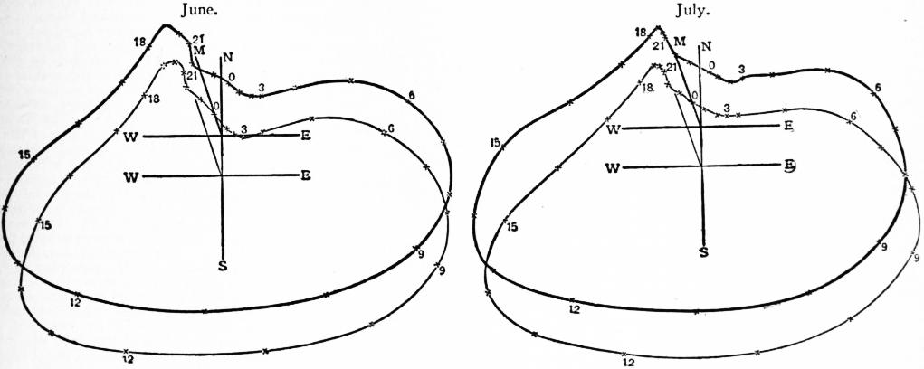
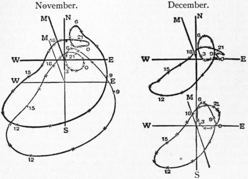
Diurnal inequalities in N and W lend themselves readily to the construction of what are known as vector diagrams. These are curves showing the direction and intensity at each hour of the day of the horizontal component of the disturbing force to which the diurnal inequality may be regarded as due. Figs. 7 and 8, taken from the Phil. Trans. vol. 204A, will serve as examples. They refer to the mean diurnal inequalities for the months stated at Kew (1890 to 1900) and Falmouth (1891 to 1902), thick lines relating to Kew, thin to Falmouth. NS and EW represent the geographical north-south and east-west directions; their intersection answers to the origin (thick lines for Kew, thin for Falmouth). The line from the origin to M represents the magnetic meridian. The line from the origin to any cross—the number indicating the corresponding hour counted from midnight as 0—represents the magnitude and direction at that hour of the horizontal component of the disturbing force to which the diurnal inequality may be assigned. The cross marks the point whose rectangular co-ordinates are the values of δN and δW derived from the diurnal inequalities of these elements. In figs. 7 and 8 the distances of the points N, E, S, W from their corresponding origin represents 10γ. The tendency to form a loop near midnight, seen in the November and December curves, is characteristic of the winter months at Kew and Falmouth. The shape is less variable in summer than in winter; but even in summer the portion answering to the hours 6 p.m. to 6 a.m. varies a good deal. The object of presenting the Kew and Falmouth curves side by side is to emphasize the close resemblance between the magnetic phenomena at places in similar latitudes, though over 200 miles apart and exhibiting widely different ranges for their meteorological elements. With considerable change of latitude however the shape of vector diagrams changes largely.

Table XV.—Diurnal Inequalities in N. and W. at Falmouth (unit 1γ).

Hour. 1 2 3 4 5 6 7 8 9 10 11 12

N. a.m. + 6 + 5 + 5 + 5 + 6 + 6 + 5 + 1 − 6 −14 −20 −20

p.m. −17 −12 − 6 − 1 + 3 + 6 + 9 + 9 + 9 + 8 + 7 + 7

W. a.m. − 2 − 2 − 3 − 4 − 6 − 9 −13 −17 −19 −13 − 3 +11

p.m. +20 +22 +17 +11 + 6 + 4 + 2 + 1 0 − 1 − 2 − 2

§ 20. Any diurnal inequality can be analysed into a series of Fourier Series. harmonic terms whose periods are 24 hours and submultiples thereof. The series may be expressed in either of the equivalent forms:—

a1 cos t + b1 sin t + a2 cos 2t + b2 sin 2t + ...

(i)

c1 sin (t + α1) + c2 sin (2t + α2) + ....

(ii)

Table XVI.—Ranges in Diurnal Inequalities at Falmouth (unit 1γ).

Jan. Feb. March. April. May. June. July. Aug. Sept. Oct. Nov. Dec.

N. 21 23 30 39 39 37 37 39 36 32 24 15

W. 20 24 46 54 55 55 54 56 51 39 24 15

In both forms t denotes time, counted usually from midnight, one hour of time being interpreted as 15° of angle. Form (i) is that utilized in actually calculating the constants a, b, ... Once the a, b, ... constants are known, the c, α, ... constants are at once derivable from the formulae:—

tan αn = an / bn; cn = an / sin αn = bn / cos αn = √(an² + bn²).

The a, b, c, α constants are called sometimes Fourier, sometimes Bessel coefficients.

(From Phil. Trans.)

Fig. 7.

By taking a sufficient number of terms a series can always be obtained which will represent any set of diurnal inequality figures; but unless one can obtain a close approach to the observational figures from the terms possessing the periods 24, 12, 8 and 6 hours the physical significance and general utility of the analysis is somewhat problematical. In the case of the magnetic elements, the 24 and 12 hour terms are usually much the more important; the 24-hour term is generally, but by no means always, the larger of the two. The c constants give the amplitudes of the harmonic terms or waves, the α constants the phase angles. An advance of 1 hour in the time of occurrence of the first (and subsequent, if any) maximum and minimum answers to an increase of 15° in α1 of 30° in α2, of 45° in α3, of 60° in α4 and so on. In the case of magnetic elements the phase angles not infrequently possess a somewhat large annual variation. It is thus essential for a minute study of the phenomena at any station to carry out the analysis for the different seasons of the year, and preferably for the individual months. If the a and b constants are known for all the individual months of one year, or for all the Januarys of a series of years, we have only to take their arithmetic means to obtain the corresponding constants for the mean diurnal inequality of the year, or for the diurnal inequality of the average January of the series of years. This, however, is obviously not true of the c or α constants, unless the phase angle is absolutely unchanged throughout the contributory months or years. This is a point requiring careful attention, because when giving values of c and α for the whole year some authorities give the arithmetic mean of the c’s and α’s calculated from the diurnal inequalities of the individual months of the year, others give the values obtained for c and α from the mean diurnal inequality of the whole year. The former method inevitably supplies a larger value for c than the latter, supposing α to vary with the season. At some observatories, e.g. Greenwich and Batavia, it has long been customary to publish every year values of the Fourier coefficients for each month, and to include other elements besides the declination. For a thoroughly satisfactory comparison of different stations, it is necessary to have data from one and the same epoch; and preferably that epoch should include at least one 11-year period. There are, however, few stations which can supply the data required for such a comparison and we have to make the best of what is available. Information is naturally most copious for the declination. For this element E. Engelenburg20 gives values of C1, C2, C3, C4, and of α1, α2, α3, α4 for each month of the year for about 50 stations, ranging from Fort Rae (62° 6′ N. lat.) to Cape Horn (55° 5′ S. lat.). From the results for individual stations, Engelenburg derives a series of means which he regards as representative of 11 different zones of latitude. His data for individual stations refer to different epochs, and some are based on only one year’s observations. The original observations also differ in reliability; thus the results are of somewhat unequal value. The mean results for Engelenburg’s zones must naturally have some of the sources of uncertainty reduced; but then the fundamental idea represented by the arrangement in zones is open to question. The majority of the data in Table XVII. are taken from Engelenburg, but the phase angles have been altered so as to apply to westerly declination. The stations are arranged in order of latitude from north to south; in a few instances results are given for quiet days. The figures represent in all cases arithmetic means derived from the 12 monthly values. In the table, so far as is known, the local mean time of the observatory has been employed. This is a point requiring attention, because most observatories employ Greenwich time, or time based on Greenwich or some other national observatory, and any departure from local time enters into the values of the constants. The data for Victoria Land refer to the “Discovery’s” 1902-1903 winter quarters, where the declination, taken westerly, was about 207°.5.

As an example of the significance of the phase angles in Table XVII., take the ordinary day data for Kew. The times of occurrence of the maxima are given by t + 234° = 450° for the 24-hour term, 2t + 39°.7 = 90° or = 450° for the 12-hour term, and so on, taking an hour in t as equivalent to 15°.

Thus the times of the maxima are:—

24-hour term, 2 h. 24 m. p.m.; 12-hour term, 1 h. 41 m. a.m. and p.m.

8-hour term, 4 h. 41 m. a.m., 0 h. 41 m. p.m., and 8 h. 41 m. p.m.

6-hour term, 0 h. 33 m. a.m. and p.m., and 6 h. 33 m. a.m. and p.m.

The minima, or extreme easterly positions in the waves, lie midway between successive maxima. All four terms, it will be seen, have maxima at some hour between 0h. 30m. and 2h. 30m. p.m. They thus reinforce one another strongly from 1 to 2 p.m., accounting for the prominence of the maximum in the early afternoon.

(From Phil. Trans.)

Fig. 8.

The utility of a Fourier analysis depends largely on whether the several terms have a definite physical significance. If the 24-hour and 12-hour terms, for instance, represent the action of forces whose distribution over the earth or whose seasonal variation is essentially different, then the analysis helps to distinguish these forces, and may assist in their being tracked to their ultimate source. Suppose, for example, one had reason to think the magnetic diurnal variation due to some meteorological phenomenon, e.g. heating of the earth’s atmosphere, then a comparison of Fourier coefficients, if such existed, for the two sets of phenomena would be a powerful method of investigation.

Table XVII.—Amplitudes and Phase Angles for Diurnal Inequality of Declination.

Place. Epoch. c1. c2. c3. c4. α1. α2. α3. α4.

′ ′ ′ ′ ° ° ° °

Fort Rae (all) 1882-1883 18.49 8.22 1.99 2.07 156.5 41.9 308 104

Fort Rae (quiet) ” 9.09 4.51 1.32 0.73 166.5 37.5 225 350

Ekatarinburg 1841-1862 2.57 1.81 0.73 0.22 223.3 7.4 204 351

Potsdam 1890-1899 2.81 1.90 0.83 0.31 239.9 32.6 237 49

Kew (ordinary) 1890-1900 2.91 1.79 0.79 0.27 234.0 39.7 239 57

Kew (quiet) ” 2.37 1.82 0.90 0.30 227.3 42.1 240 55

Falmouth (quiet) 1891-1902 2.18 1.82 0.91 0.29 226.2 40.5 238 56

Parc St Maur 1883-1899 2.70 1.87 0.85 0.30 238.6 32.5 235 95

Toronto 1842-1848 2.65 2.34 1.00 0.33 213.7 34.9 238 350

Washington 1840-1842 2.38 1.86 0.65 0.33 223.0 26.6 223 53

Manila 1890-1900 0.53 0.58 0.43 0.17 266.3 50.7 226 89

Trivandrum 1853-1864 0.54 0.46 0.29 0.10 289.0 49.6 114

Batavia 1883-1899 0.80 0.88 0.43 0.13 332.0 163.2 5 236

St. Helena 1842-1847 0.68 0.61 0.63 0.34 275.8 171.4 27 244

Mauritius 1876-1890 0.86 1.11 0.76 0.22 21.6 172.7 350 161

C. of G. Hope 1841-1846 1.15 1.13 0.80 0.35 287.7 156.0 351 193

Melbourne 1858-1863 2.52 2.45 1.23 0.35 27.4 176.7 9 193

Hobart 1841-1848 2.29 2.15 0.87 0.32 33.6 170.8 349 185

S. Georgia 1882-1883 2.13 1.28 0.76 0.31 30.3 185.3 7 180

Victoria Land (all) 1902-1903 20.51 4.81 1.21 1.32 158.7 306.9 292 303

Victoria Land (quieter) ” 15.34 4.05 1.24 1.18 163.8 312.9 261

§ 21. Fourier coefficients of course often vary much with the season of the year. In the case of the declination this is especially true of the phase angles at tropical stations. To enter on details for a number of stations would unduly occupy space. A fair idea of the variability in the case of declination in temperate latitudes may be derived from Table XVIII., which gives monthly values for Kew derived from ordinary days of an 11-year period 1890-1900.

Fourier analysis has been applied to the diurnal inequalities of the other magnetic elements, but more sparingly. Such results are illustrated by Table XIX., which contains data derived from quiet days at Kew from 1890 to 1900. Winter includes November to February, Summer May to August, and Equinox the remaining four months. In this case the data are derived from mean diurnal inequalities for the season specified. In the case of the c or amplitude coefficients the unit is 1′ for I (inclination), and 1γ for H and V (horizontal and vertical force). At Kew the seasonal variation in the amplitude is fairly similar for all the elements. The 24-hour and 12-hour terms tend to be largest near midsummer, and least near midwinter; but the 8-hour and 6-hour terms have two well-marked maxima near the equinoxes, and a clearly marked minimum near midsummer, in addition to one near midwinter. On the other hand, the phase angle phenomena vary much for the different elements. The 24-hour term, for instance, has its maximum earlier in winter than in summer in the case of the declination and vertical force, but the exact reverse holds for the inclination and the horizontal force.

Table XVIII.—Kew Declination: Amplitudes and Phase Angles (local mean time).

Month. c1. c2. c3. c4. α1. α2. α3. α4.

′ ′ ′ ′ ° ° ° °

January 1.79 0.86 0.41 0.27 251.2 29.8 254 64

February 2.41 1.11 0.57 0.30 242.0 27.7 235 39

March 3.05 1.98 1.11 0.45 233.2 36.1 223 49

April 3.35 2.48 1.17 0.39 224.8 39.2 228 61

May 3.57 2.38 0.87 0.17 221.3 50.8 245 89

June 3.83 2.39 0.74 0.05 212.6 46.7 239 72

July 3.72 2.30 0.77 0.11 214.6 48.1 233 8

August 3.64 2.43 1.05 0.18 228.2 57.2 244 51

September 3.35 2.02 1.04 0.35 236.9 55.3 245 70

October 2.69 1.69 0.92 0.48 240.1 35.6 235 65

November 1.94 1.06 0.51 0.32 248.3 28.3 247 61

December 1.61 0.81 0.35 0.20 255.1 22.0 243 56

§ 22. If secular change proceeded uniformly throughout the year, the value En of any element at the middle of the nth month of the year would be connected with E, the mean value for the whole year, by the formula En = E + (2n − 13)s/24, Annual Inequality. where s is the secular change per annum. For the present purpose, difference in the lengths of the months may be neglected. If one applies to En − E the correction −(2n − 13)s/24 one eliminates a regularly progressive secular change; what remains is known as the annual inequality. If only a short period of years is dealt with, irregularities in the secular change from year to year, or errors of observation, may obviously simulate the effect of a real annual inequality. Even when a long series of years is included, there is always a possibility of a spurious inequality arising from annual variation in the instruments, or from annual change in the conditions of observation. J. Liznar,21 from a study of data from a number of stations, arrived at certain mean results for the annual inequalities in declination and inclination in the northern and southern hemispheres, and J. Hann22 has more recently dealt with Liznar’s and newer results. Table XX. gives a variety of data, including the mean results given by Liznar and Hann. In the case of declination + denotes westerly position; in the case of inclination it denotes a larger dip (whether the inclination be north or south). According to Liznar declination in summer is to the west of the normal position in both hemispheres. The phenomena, however, at Parc St Maur are, it will be seen, the exact opposite of what Liznar regards as normal; and whilst the Potsdam results resemble his mean in type, the range of the inequality there, as at Parc St Maur, is relatively small. Of the three sets of data given for Kew the first two are derived in a similar way to those for other stations; the first set are based on quiet days only, the second on all but highly disturbed days. Both these sets of results are fairly similar in type to the Parc St Maur results, but give larger ranges; they are thus even more opposed to Liznar’s normal type. The last set of data for Kew is of a special kind. During the 11 years 1890 to 1900 the Kew declination magnetograph showed to within 1′ the exact secular change as derived from the absolute observations; also, if any annual variation existed in the position of the base lines of the curves it was exceedingly small. Thus the accumulation of the daily non-cyclic changes shown by the curves should closely represent the combined effects of secular change and annual inequality. Eliminating the secular change, we arrive at an annual inequality, based on all days of the year including the highly disturbed. It is this annual inequality which appears under the heading s. It is certainly very unlike the annual inequality derived in the usual way. Whether the difference is to be wholly assigned to the fact that highly disturbed days contribute in the one case, but not in the other, is a question for future research.

Table XIX.—Kew Diurnal Inequality: Amplitudes and Phase Angles (local mean time).

c1. c2. c3. c4. α1. α2. α3. α4.

° ° ° °

I Winter 0.240 0.222 0.104 0.076 250.0 91.8 344 194

Equinox 0.601 0.290 0.213 0.127 290.3 135.5 4 207

Summer 0.801 0.322 0.172 0.070 312.5 155.5 39 238

H Winter 3.62 3.86 1.81 1.13 82.9 277.3 154 6

Equinox 10.97 5.87 3.32 1.84 109.6 303.5 167 16

Summer 14.85 6.23 2.35 0.95 130.3 316.5 199 41

V Winter 2.46 1.67 0.86 0.42 153.9 300.8 108 280

Equinox 6.15 4.70 2.51 0.94 117.2 272.3 99 289

Summer 8.63 6.45 2.24 0.55 122.0 272.4 100 285

In the case of the inclination, Liznar found that in both hemispheres the dip (north in the northern, south in the southern hemisphere) was larger than the normal when the sun was in perihelion, corresponding to an enhanced value of the horizontal force in summer in the northern hemisphere.

In the case of annual inequalities, at least that of the declination, it is a somewhat suggestive fact that the range seems to become less as we pass from older to more recent results, or from shorter to longer periods of years. Thus for Paris from 1821 to 1830 Arago deduced a range of 2′ 9″. Quiet days at Kew from 1890 to 1894 gave a range of 1′.2, while at Potsdam Lüdeling got a range 30% larger than that in Table XX. when considering the shorter period 1891-1899. Up to the present, few individual results, if any, can claim a very high degree of certainty. With improved instruments and methods it may be different in the future.

Table XX.—Annual Inequality.

Declination. Inclination.

Liznar, N. Hemi- sphere. Potsdam, 1891-1906. Parc St Maur, 1888-1897. Kew (1890-1900). Batavia, 1883-1893. Mauritius. Liznar & Hann’s mean. Potsdam. Parc St. Maur. Kew.

q. o. s.

′ ′ ′ ′ ′ ′ ′ ′ ′ ′ ′ ′

January −0.25 +0.04 +0.01 +0.08 +0.03 +0.32 +0.23 +0.06 +0.49 +0.32 +0.44 −0.03

February −0.54 −0.11 0.00 +0.48 +0.25 −0.20 +0.19 +0.29 +0.39 +0.56 +0.29 −0.07

March −0.27 +0.04 +0.17 +0.03 +0.05 −1.02 −0.12 +0.27 +0.20 +0.38 +0.13 +0.53

April −0.03 +0.10 +0.12 −0.31 −0.14 −0.90 −0.11 +0.30 −0.08 −0.02 −0.13 +0.18

May +0.19 +0.07 −0.11 −0.39 −0.28 +0.29 −0.30 +0.08 −0.43 −0.29 −0.37 −0.15

June +0.46 +0.13 −0.14 −0.47 −0.39 +0.78 −0.13 −0.19 −0.70 −0.77 −0.59 −0.35

July +0.48 +0.14 −0.17 −0.30 −0.13 +0.44 −0.08 −0.44 −0.72 −0.67 −0.27 −0.13

August +0.47 +0.11 +0.01 +0.08 +0.05 +0.52 −0.18 −0.38 −0.47 −0.23 −0.05 −0.19

September +0.31 +0.01 0.00 +0.29 +0.24 −0.02 +0.06 −0.06 −0.06 +0.16 +0.01 +0.20

October −0.07 −0.11 +0.09 +0.06 +0.01 −0.26 +0.03 −0.04 +0.31 +0.27 +0.19 0.00

November −0.30 −0.28 −0.05 +0.17 +0.11 −0.02 +0.08 −0.01 +0.51 +0.30 +0.43 +0.18

December −0.36 −0.14 +0.05 +0.26 +0.23 +0.05 +0.35 +0.06 +0.55 +0.19 +0.24 −0.29

Range 1.02 0.42 0.34 0.95 0.64 1.80 0.65 0.74 1.27 1.33 1.03 0.88

§ 23. The inequalities in Table XX. may be analysed—as has in fact been done by Hann—in a series of Fourier terms, whose periods are the year and its submultiples. Fourier series can also be formed representing the annual variation in the Annual Variation Fourier Coefficients. amplitudes of the regular diurnal inequality, and its component 24-hour, 12-hour, &c. waves, or of the amplitude of the absolute daily range (§ 24). To secure the highest theoretical accuracy, it would be necessary in calculating the Fourier coefficients to allow for the fact that the “months” from which the observational data are derived are not of uniform length. The mid-times, however, of most months of the year are but slightly displaced from the position they would occupy if the 12 months were exactly equal, and these displacements are usually neglected. The loss of accuracy cannot be but trifling, and the simplification is considerable.

The Fourier series may be represented by

P1 sin (t + θ1) + P2 sin (2t + θ2) + ...,

where t is time counted from the beginning of the year, one month being taken as the equivalent of 30°, P1, P2 represent the amplitudes, and θ1, θ2 the phase angles of the first two terms, whose periods are respectively 12 and 6 months. Table XXI. gives the values of these coefficients in the case of the range of the regular diurnal inequality for certain specified elements and periods at Kew23 and Falmouth.23a In the case of P1 and P2 the unit is 1′ for D and I, and 1γ for H and V. M denotes the mean value of the range for the 12 months. The letters q and o represent quiet and ordinary day results. S max. means the years 1892-1895, with a mean sun spot frequency of 75.0. S min. for Kew means the years 1890, 1899 and 1900 with a mean sun spot frequency of 9.6; for Falmouth it means the years 1899-1902 with a mean sun spot frequency of 7.25.

Increase in θ1 or θ2 means an earlier occurrence of the maximum or maxima, 1° answering roughly to one day in the case of the 12-month term, and to half a day in the case of the 6-month term. P1/M and P2/M both increase decidedly as we pass from years of many to years of few sun spots; i.e. relatively considered the range of the regular diurnal inequality is more variable throughout the year when sun spots are few than when they are many.

The tendency to an earlier occurrence of the maximum as we pass from quiet days to ordinary days, or from years of sun spot minimum to years of sun spot maximum, which appears in the table, appears also in the case of the horizontal force—at least in the case of the annual term—both at Kew and Falmouth. The phenomena at the two stations show a remarkably close parallelism. At both, and this is true also of the absolute ranges, the maximum of the annual term falls in all cases near midsummer, the minimum near midwinter. The maxima of the 6-month terms fall near the equinoxes.

Table XXI.—Annual Variation of Diurnal Inequality Range. Fourier Coefficients.

P1. P2. θ1. θ2. P1/M. P2/M.

Kew Do 3.36 0.94 279° 280° 0.40 0.11

1890-1900 Dq 3.81 1.22 275° 273° 0.47 0.15

Iq 0.67 0.16 264° 269° 0.42 0.10

Hq 13.6 3.0 269° 261° 0.48 0.11

Vq 11.7 2.2 282° 242° 0.63 0.12

S max. Kew 4.50 1.26 277° 282° 0.47 0.13

Dq Falmouth 4.10 1.40 277° 286° 0.43 0.15

S min. Kew 3.35 1.10 274° 269° 0.49 0.16

Dq Falmouth 3.19 1.14 275° 277° 0.49 0.17

§ 24. Allusion has already been made in § 14 to one point which requires fuller discussion. If we take a European station such as Kew, the general character of, say, the declination does not vary very much with the season, but still it does Absolute Range. vary. The principal minimum of the day, for instance, occurs from one to two hours earlier in summer than in winter. Let us suppose for a moment that all the days of a month are exactly alike, the difference in type between successive months coming in per saltum. Suppose further that having formed twelve diurnal inequalities from the days of the individual months of the year, we deduce a mean diurnal inequality for the whole year by combining these twelve inequalities and taking the mean. The hours of maximum and minimum being different for the twelve constituents, it is obvious that the resulting maximum will normally be less than the arithmetic mean of the twelve maxima, and the resulting minimum (arithmetically) less than the arithmetic mean of the twelve minima. The range—or algebraic excess of the maximum over the minimum—in the mean diurnal inequality for the year is thus normally less than the arithmetic mean of the twelve ranges from diurnal inequalities for the individual months. Further, as we shall see later, there are differences in type not merely between the different months of the year, but even between the same months in different years. Thus the range of the mean diurnal inequality for, say, January based on the combined observations of, say, eleven Januarys may be and generally will be slightly less than the arithmetic mean of the ranges obtained from the Januarys separately. At Kew, for instance, taking the ordinary days of the 11 years 1890-1900, the arithmetic mean of the diurnal inequality ranges of declination from the 132 months treated independently was 8′.52, the mean range from the 12 months of the year (the eleven Januarys being combined into one, and so on) was 8′.44, but the mean range from the whole 4,000 odd days superposed was only 8′.03. Another consideration is this: a diurnal inequality is usually based on hourly readings, and the range deduced is thus an under-estimate unless the absolute maximum and minimum both happen to come exactly at an hour. These considerations would alone suffice to show that the absolute range in individual days, i.e. the difference between the algebraically largest and least values of the element found any time during the 24 hours, must on the average exceed the range in the mean diurnal inequality for the year, however this latter is formed. Other causes, moreover, are at work tending in the same direction. Even in central Europe, the magnetic curves for individual days of an ordinary month often differ widely amongst themselves, and show maxima and minima at different times of the day. In high latitudes, the variation from day to day is sometimes so great that mere eye inspection of magnetograph curves may leave one with but little idea as to the probable shape of the resultant diurnal curve for the month. Table XXII. gives the arithmetic mean of the absolute daily ranges from a few stations. The values which it assigns to the year are the arithmetic means of the 12 monthly values. The Mauritius data are for different periods, viz. declination 1875, 1880 and 1883 to 1890, horizontal force 1883 to 1890, vertical force 1884 to 1890. The other data are all for the period 1890 to 1900.

Table XXII.—Mean Absolute Daily Ranges (Units 1′ for Declination, 1γ for H and V).

Jan. Feb. Mar. April. May. June. July. Aug. Sept. Oct. Nov. Dec. Year.

Declination.

Pavlovsk 13.42 17.20 18.22 17.25 17.76 15.91 16.89 16.57 16.75 15.70 13.87 12.37 15.99

Ekatarinburg 7.33 9.54 11.90 12.89 13.63 13.03 12.78 12.21 11.23 9.44 7.86 6.85 10.72

Kew. All days 11.16 13.69 15.93 15.00 14.90 13.65 14.13 14.22 14.57 14.07 11.71 9.80 13.57

Kew. Ordinary days 10.14 11.87 14.19 14.24 13.85 13.26 13.47 13.67 13.71 13.10 10.40 9.00 12.58

Kew. Quiet days 6.12 7.57 10.59 11.84 12.09 11.95 11.60 11.93 10.86 9.16 6.54 5.08 9.61

Zi-ka-wei 3.88 3.25 6.22 7.04 7.15 7.40 7.77 8.06 6.73 4.68 2.91 2.52 5.63

Mauritius 6.93 7.79 7.11 5.75 4.87 4.03 4.36 6.00 6.28 6.71 6.99 6.78 6.13

Horizontal force.

Pavlovsk 52.4 74.5 79.1 80.1 86.2 79.0 86.7 77.6 76.7 67.3 55.7 45.9 71.8

Ekatarinburg 33.2 43.1 48.4 51.7 56.2 54.1 56.7 51.7 49.3 44.1 34.1 29.3 46.0

Mauritius 37.9 35.0 36.2 37.6 35.0 34.1 33.8 34.5 36.6 37.4 37.8 35.3 35.9

Vertical force.

Pavlovsk 27.0 50.4 54.7 43.2 45.3 34.8 42.1 35.5 42.5 37.5 33.5 25.5 39.3

Ekatarinburg 17.4 26.6 29.2 30.1 29.6 27.6 29.6 26.1 25.2 22.1 19.6 16.4 24.9

Mauritius 17.1 19.5 20.1 17.3 16.5 15.5 17.1 22.0 22.7 19.4 16.7 15.2 18.2

A comparison of the absolute ranges in Table XXII. with the inequality ranges for the same stations derivable from Tables VIII. to X. is most instructive. At Mauritius the ratio of the absolute to the inequality range is for D 1.38, for H 1.76, and for V 1.19. At Pavlovsk the corresponding ratios are much larger, viz. 2.16 for D, 2.43 for H, and 2.05 for V. The declination data for Kew in Table XXII. illustrate other points. The first set of data are derived from all days of the year. The second omit the highly disturbed days. The third answer to the 5 days a month selected as typically quiet. The yearly mean absolute range from ordinary days at Kew in Table XXII. is 1.49 times the mean inequality range in Table VIII.; comparing individual months the ratio of the absolute to the inequality range varies from 2.06 in January to 1.21 in June. Even confining ourselves to the quiet days at Kew, which are free from any but the most trifling disturbances, we find that the mean absolute range for the year is 1.20 times the arithmetic mean of the inequality ranges for the individual months of the year, and 1.22 times the range from the mean diurnal inequality for the year. In this case the ratio of the absolute to the inequality range varies from 1.55 in December to only 1.09 in May.

§ 25. The variability of the absolute daily range of declination is illustrated by Table XXIII., which contains data for Kew24 derived from all days of the 11-year period 1890-1900. It gives the total number of times during the 11 years when the absolute range lay within the limits specified at the heads of the first nine columns of figures. The two remaining columns give the arithmetic means of the five largest and the five least absolute ranges encountered each month. The mean of the twelve monthly diurnal inequality ranges from ordinary days was only 8′.44, but the absolute range during the 11 years exceeded 20′ on 492 days, 15′ on 1196 days, and 10′ on 2784 days, i.e. on 69 days out of every 100.

Table XXIII.—Absolute Daily Range of Declination at Kew.

Number of occasions during 11 years when absolute range was:— Means from the 5 largest and 5 least ranges of the month on the average of 11 years.

0′ to 5′. 5′ to 10′. 10′ to 15′. 15′ to 20′. 20′ to 25′. 25′ to 30′. 30′ to 35′. 35′ to 40′. over 40′. 5 largest. 5 least.

′ ′

January 51 145 69 37 24 7 4 3 1 22.90 5.07

February 26 99 84 51 26 10 4 2 8 27.21 6.55

March 1 72 138 61 32 21 8 1 7 29.87 8.93

April 0 43 167 73 27 10 6 3 1 23.69 10.31

May 0 57 157 85 20 12 3 0 7 25.36 9.50

June 0 56 185 67 15 1 3 1 2 19.92 9.89

July 0 59 185 70 14 5 2 2 4 22.49 9.96

August 0 37 202 75 22 1 2 0 2 21.27 10.05

September 1 68 153 71 19 5 4 5 4 24.55 9.52

October 3 103 111 67 34 10 11 2 0 23.92 8.01

November 42 140 81 28 14 9 8 5 3 23.58 5.64

December 64 166 56 29 14 7 1 1 3 20.43 4.36

Totals 188 1045 1588 714 261 98 56 25 42

§ 26. Magnetic phenomena, both regular and irregular, at any station vary from year to year. The extent of this variation is illustrated in Tables XXIV. and XXV., both relating to the period 1890 to 1900.25 Table XXIV. gives the amplitudes of Relations to Sun-spot Frequency. the regular diurnal inequality in the elements stated at the head of the columns. The ordinary day declination data (D0) for Kew represent arithmetic means from the twelve months of the year; the other data all answer to the mean diurnal inequality for the whole year. Table XXV. gives the arithmetic means for each year of the absolute daily range, of the monthly range (or difference between the highest and lowest values in the month), and of the yearly range (or difference between the highest and lowest values of the year). The numerals attached to the years in these tables indicate their order as regards sun-spot frequency according to Wolf and Wolfer (see Aurora Polaris), 1893 being the year of largest frequency, and 1890 that of least. The difference in sun-spot frequency between 1897 and 1898 was microscopic; the differences between 1890, 1900 and 1899 were small, and those between 1893, 1894 and 1892 were not very large.

The years 1892-1895 represent high sun-spot frequency, while 1890, 1899 and 1900 represent low frequency. Table XXIV. shows that 1892 to 1895 were in all cases distinguished by the large size of the inequality ranges, and 1890, 1899 and 1900 by the small size. The range in 1893 is usually the largest, and though the H and V ranges at Ekaterinburg are larger in 1892 than in 1893, the excess is trifling. The phenomena apparent in Table XXIV. are fairly representative; other stations and other periods associate large inequality ranges with high sun-spot frequency. The diurnal inequality range it should be noticed is comparatively little influenced by irregular disturbances. Coming to Table XXV., we have ranges of a different character. The absolute range at Kew on quiet days is almost as little influenced by irregularities as is the range of the diurnal inequality, and in its case the phenomena are very similar to those observed in Table XXIV. As we pass from left to right in Table XXV., the influence of disturbance increases. Simultaneously with this, the parallelism with sun-spot frequency is less close. The entries relating to 1892 and 1894 become more and more prominent compared to those for 1893. The yearly range may depend on but a single magnetic storm, the largest disturbance of the year possibly far outstripping any other. But taking even the monthly ranges the values for 1893 are, speaking roughly, only half those for 1892 and 1894, and very similar to those of 1898, though the sun-spot frequency in the latter year was less than a third of that in 1893. Ekatarinburg data exactly analogous to those for Pavlovsk show a similar prominence in 1892 and 1894 as compared to 1893. The retirement of 1893 from first place, seen in the absolute ranges at Kew, Pavlovsk and Ekatarinburg, is not confined to the northern hemisphere. It is visible, for instance, in the amplitudes of the Batavia disturbance results. Thus though the variation from year to year in the amplitude of the absolute ranges is relatively not less but greater than that of the inequality ranges, and though the general tendency is for all ranges to be larger in years of many than in years of few sun-spots, still the parallelism between the changes in sun-spot frequency and in magnetic range is not so close for the absolute ranges and for disturbances as for the inequality ranges.

Table XXIV.—Ranges of Diurnal Inequalities.

Pavlovsk. Ekatarinburg. Kew.

D. I. H. D. I. H. V. Dq. Iq. Hq. Do.

′ ′ γ ′ ′ γ γ ′ ′ γ ′

189011 6.32 1.33 22 5.83 1.05 18 9 6.90 20 7.32

18916 7.31 1.79 30 6.85 1.38 25 14 8.04 1.52 28 8.48

18923 8.75 2.21 37 7.74 1.72 32 19 9.50 1.66 31 9.85

18931 9.64 2.24 38 8.83 1.80 31 17 10.06 1.96 35 10.74

18942 8.58 2.17 38 7.80 1.73 30 17 9.32 1.94 34 9.80

18954 8.22 2.08 33 7.29 1.64 28 15 8.59 1.66 30 9.54

18965 7.39 1.77 29 6.50 1.38 25 15 7.77 1.31 25 8.50

18976 6.79 1.59 26 6.01 1.16 21 12 6.71 1.14 22 7.76

18987 6.25 1.56 26 5.76 1.19 21 11 6.85 1.07 21 7.59

18999 6.02 1.44 24 5.33 1.12 20 11 6.69 1.01 21 7.30

190010 6.20 1.28 22 5.88 0.93 17 8 6.52 1.06 21 6.83

Table XXV.—Absolute Ranges.

Kew Declination. Daily. Pavlovsk.

Daily. Monthly. Yearly.

q. o. a. D. H. V. D. H. V. D. H. V.

′ ′ ′ ′ γ γ ′ γ γ ′ γ γ

189011 8.3 10.5 10.7 12.1 49 21 28.2 118 80 42.1 169 179

18916 10.0 12.8 13.7 16.0 70 39 46.3 218 233 92.3 550 614

18923 12.3 15.4 17.7 21.0 111 73 93.6 698 575 194.0 2416 1385

18931 11.8 15.2 15.6 17.8 79 41 48.3 241 210 87.1 514 457

18942 11.3 14.7 16.5 20.4 97 62 84.1 493 493 145.6 1227 878

18954 10.6 14.8 15.6 18.1 80 46 47.4 220 223 73.9 395 534

18965 9.5 12.9 14.5 17.5 74 43 52.4 232 236 88.7 574 608

18978 8.2 11.5 12.1 14.6 61 30 43.8 201 170 101.1 449 480

18987 8.2 11.2 12.3 14.7 67 35 46.6 276 242 118.9 1136 888

18999 7.9 10.5 11.3 13.1 58 27 38.3 178 150 63.8 382 527

190010 7.4 8.9 9.2 10.5 44 16 32.8 134 89 94.2 457 365

Means 9.6 12.6 13.6 16.0 72 39 51.1 274 246 100.2 752 629

§ 27. The relationship between magnetic ranges and sun-spot frequency has been investigated in several ways. W. Ellis26 has employed a graphical method which has advantages, especially for tracing the general features of the resemblance, and is besides independent of any theoretical hypothesis. Taking time for the axis of abscissae, Ellis drew two curves, one having for its ordinates the sun-spot frequency, the other the inequality range of declination or of horizontal force at Greenwich. The value assigned in the magnetic curve to the ordinate for any particular month represents a mean from 12 months of which it forms a central month, the object being to eliminate the regular annual variation in the diurnal inequality. The sun-spot data derived from Wolf and Wolfer were similarly treated. Ellis originally dealt with the period 1841 to 1877, but subsequently with the period 1878 to 1896, and his second paper gives curves representing the phenomena over the whole 56 years. This period covered five complete sun-spot periods, and the approximate synchronism of the maxima and minima, and the general parallelism of the magnetic and sun-spot changes is patent to the eye. Ellis27 has also applied an analogous method to investigate the relationship between sun-spot frequency and the number of days of magnetic disturbance at Greenwich. A decline in the number of the larger magnetic storms near sun-spot minimum is recognizable, but the application of the method is less successful than in the case of the inequality range. Another method, initiated by Professor Wolf of Zurich, lends itself more readily to the investigation of numerical relationships. He started by supposing an exact proportionality between corresponding changes in sun-spot frequency and magnetic range. This is expressed mathematically by the formula

R = a + bS ≡ a {1 + (b/a) S },

where R denotes the magnetic range, S the corresponding sun-spot frequency, while a and b are constants. The constant a represents the range for zero sun-spot frequency, while b/a is the proportional increase in the range accompanying unit rise in sun-spot frequency. Assuming the formula to be true, one obtains from the observed values of R and S numerical values for a and b, and can thus investigate whether or not the sun-spot influence is the same for the different magnetic elements and for different places. Of course, the usefulness of Wolf’s formula depends largely on the accuracy with which it represents the facts. That it must be at least a rough approximation to the truth in the case of the diurnal inequality at Greenwich might be inferred from Ellis’s curves. Several possibilities should be noticed. The formula may apply with high accuracy, a and b having assigned values, for one or two sun-spot cycles, and yet not be applicable to more remote periods. There are only three or four stations which have continuous magnetic records extending even 50 years back, and, owing to temperature correction uncertainties, there is perhaps no single one of these whose earlier records of horizontal and vertical force are above criticism. Declination is less exposed to uncertainty, and there are results of eye observations of declination before the era of photographic curves. A change, however, of 1′ in declination has a significance which alters with the intensity of the horizontal force. During the period 1850-1900 horizontal force in England increased about 5%, so that the force requisite to produce a declination change of 19′ in 1900 would in 1850 have produced a deflection of 20′. It must also be remembered that secular changes of declination must alter the angle between the needle and any disturbing force acting in a fixed direction. Thus secular alteration in a and b is rather to be anticipated, especially in the case of the declination. Wolf’s formula has been applied by Rajna28 to the yearly mean diurnal declination ranges at Milan based on readings taken twice daily from 1836 to 1894, treating the whole period together, and then the period 1871 to 1894 separately. During two sub-periods, 1837-1850 and 1854-1867, Rajna’s calculated values for the range differ very persistently in one direction from those observed; Wolf’s formula was applied by C. Chree25 to these two periods separately. He also applied it to Greenwich inequality ranges for the years 1841 to 1896 as published by Ellis, treating the whole period and the last 32 years of it separately, and finally to all (a) and quiet (q) day Greenwich ranges from 1889 to 1896. The results of these applications of Wolf’s formula appear in Table XXVI.

The Milan results are suggestive rather of heterogeneity in the material than of any decided secular change in a or b. The Greenwich data are suggestive of a gradual fall in a, and rise in b, at least in the case of the declination.

Table XXVII. gives values of a, b and b/a in Wolf’s formula calculated by Chree25 for a number of stations. There are two sets of data, the first set relating to the range from the mean diurnal inequality for the year, the second to the arithmetic mean of the ranges in the mean diurnal inequalities for the twelve months. It is specified whether the results were derived from all or from quiet days.

Table XXVI.—Values of a and b in Wolf’s Formula.

Milan. Greenwich.

Epoch. Declination (unit 1′). Epoch. Declination (unit 1′). Horizontal Force (unit 1γ).

a. b. a. b. a. b.

1836-94 5.31 .047 1841-96 7.29 .0377 26.4 .190

1871-94 5.39 .047 1865-96 7.07 .0396 23.6 .215

1837-50 6.43 .041 1889-96(a) 6.71 .0418 23.7 .218

1854-67 4.62 .047 1889-96(q) 6.36 .0415 25.0 .213

As explained above, a would represent the range in a year of no sun-spots, while 100 b would represent the excess over this shown by the range in a year when Wolf’s sun-spot frequency is 100. Thus b/a seems the most natural measure of sun-spot influence. Accepting it, we see that sun-spot influence appears larger at most places for inclination and horizontal force than for declination. In the case of vertical force there is at Pavlovsk, and probably in a less measure at other northern stations, a large difference between all and quiet days, which is not shown in the other elements. The difference between the values of b/a at different stations is also exceptionally large for vertical force. Whether this last result is wholly free from observational uncertainties is, however, open to some doubt, as the agreement between Wolf’s formula and observation is in general somewhat inferior for vertical force. In the case of the declination, the mean numerical difference between the observed values and those derived from Wolf’s formula, employing the values of a and b given in Table XXVII., represented on the average about 4% of the mean value of the element for the period considered, the probable error representing about 6% of the difference between the highest and lowest values observed. The agreement was nearly, if not quite, as good as this for inclination and horizontal force, but for vertical force the corresponding percentages were nearly twice as large.

Table XXVII.—Values of a and b in Wolf’s Formula.

Declination(unit 1′). Inclination (unit 1′). Horizontal Force (unit 1γ). Vertical Force (unit 1γ).

Diurnal Inequality for the Year. a. b. 100 b/a. a. b. 100 b/a. a. b. 100 b/a. a. b. 100 b/a.

Pavlovsk, 1890-1900 all 5.74 .0400 .70 1.24 .0126 1.01 20.7 .211 1.02 8.1 .265 3.26

Pavlovsk, 1890-1900 quiet 6.17 .0424 .69 · · · · · · 20.6 .195 0.95 5.9 .027 0.46

Ekatarinburg, 1890-1900 all 5.29 .0342 .65 0.93 .0105 1.13 16.8 .182 1.09 8.6 .117 1.37

Irkutsk , 1890-1900 all 4.82 .0358 .74 0.97 .0087 0.90 18.2 .190 1.04 6.5 .071 1.09

Kew, 1890-1900 quiet 6.10 .0433 .71 0.87 .0125 1.45 18.1 .194 1.07 14.3 .081 0.56

Falmouth, 1891-1902 quiet 5.90 .0451 .76 · · · · · · 20.1 .233 1.16 · · · · · ·

Kolaba, 1894-1901 quiet 2.37 .0066 .28 · · · · · · 31.6 .281 0.89 19.4 .072 0.37

Batavia, 1887-1898 all 2.47 .0179 .72 3.60 .0218 0.61 38.7 .274 0.71 30.1 .156 0.52

Mauritius 1875-1880 1883-1890 all 4.06 .0164 .40 · · · · · · 15.0 .096 0.64 11.9 .069 0.58

Mean from individual months:—

Pavlovsk, 1890-1900 all 6.81 .0446 .66 1.44 .0151 1.05 22.8 .243 1.07 9.7 .287 2.97

Pavlovsk, 1890-1900 quiet 6.52 .0442 .68 · · · · · · 22.2 .208 0.94 7.0 .044 0.63

Ekatarinburg, 1890-1900 all 6.18 .0355 .58 1.12 .0120 1.06 19.2 .195 1.01 9.2 .156 1.70

Greenwich, 1865-1896 all 7.07 .0396 .56 · · · · · · 23.6 .215 0.91 · · · · · ·

Kew, 1890-1900 all 6.65 .0428 .64 · · · · · · · · · · · · · · · · · ·

Kew, 1890-1900 quiet 6.49 .0410 .63 1.17 .0130 1.11 21.5 .191 0.89 16.0 .072 0.45

Falmouth, 1891-1902 quiet 6.16 .0450 .73 · · · · · · 20.9 .236 1.13 · · · · · ·

Applying Wolf’s formula to the diurnal ranges for different months of the year, Chree found, as was to be anticipated, that the constant a had an annual period, with a conspicuous minimum at midwinter; but whilst b also varied, it did so to a much less extent, the consequence being that b/a showed a minimum at midsummer. The annual variation in b/a alters with the place, with the element, and with the type of day from which the magnetic data are derived. Thus, in the case of Pavlovsk declination, whilst the mean value of 100 b/a for the 12 months is, as shown in Table XXVII., 0.66 for all and 0.68 for quiet days—values practically identical—if we take the four midwinter and the four midsummer months separately, we have 100 b/a, varying from 0.81 in winter to 0.52 in summer on all days, but from 1.39 in winter to 0.52 in summer on quiet days. In the case of horizontal force at Pavlovsk the corresponding figures to these are for all days—winter 1.77, summer 0.98, but for quiet days—winter 1.83, summer 0.71.

Wolf’s formula has also been applied to the absolute daily ranges, to monthly ranges, and to various measures of disturbance. In these cases the values found for b/a are usually larger than those found for diurnal inequality ranges, but the accordance between observed values and those calculated from Wolf’s formula is less good. If instead of the range of the diurnal inequality we take the sum of the 24-hourly differences from the mean for the day—or, what comes to the same thing, the average departure throughout the 24 hours from the mean value for the day—we find that the resulting Wolf’s formula gives at least as good an agreement with observation as in the case of the inequality range itself. The formulae obtained in the case of the 24 differences, at places as wide apart as Kew and Batavia, agreed in giving a decidedly larger value for b/a than that obtained from the ranges. This indicates that the inequality curve is relatively less peaked in years of many than in years of few sun-spots.

§ 28. The applications of Ellis’s and Wolf’s methods relate directly only to the amplitude of the diurnal changes. There is, however, a change not merely in amplitude but in type. This is clearly seen when we compare the values found in years of many and of few sun-spots for the Fourier coefficients in the diurnal inequality. Such a comparison is carried out in Table XXVIII. for the declination on ordinary days at Kew. Local mean time is used. The heading S max. (sun-spot maximum) denotes mean average results from the four years 1892-1895, having a mean sun-spot frequency of 75.0, whilst S min. (sun-spot minimum) applies similarly to the years 1890, 1899 and 1900, having a mean sun-spot frequency of only 9.6. The data relate to the mean diurnal inequality for the whole year or for the season stated. It will be seen that the difference between the c, or amplitude, coefficients in the S max. and S min. years is greater for the 24-hour term than for the 12-hour term, greater for the 12-hour than for the 8-hour term, and hardly apparent in the 6-hour term. Also, relatively considered, the difference between the amplitudes in S max. and S min. years is greatest in winter and least in summer. Except in the case of the 6-hour term, where the differences are uncertain, the phase angle is larger, i.e. maxima and minima occur earlier in the day, in years of S min. than in years of S max. Taking the results for the whole year in Table XXVIII., this advance of phase in the S min. years represents in time 15.6 minutes for the 24-hour term, 9.4 minutes for the 12-hour term, and 14.7 minutes for the 8-hour term. The difference in the phase angles, as in the amplitudes, is greatest in winter. Similar phenomena are shown by the horizontal force, and at Falmouth24 as well as Kew.

Table XXVIII.—Fourier Coefficients in Years of many and few Sun-spots.

Year. Winter. Equinox. Summer.

S max. S min. S max. S min. S max. S min. S max. S min.

′ ′ ′ ′ ′ ′ ′ ′

c1 3.47 2.21 2.41 1.43 3.76 2.41 4.38 2.98

c2 2.04 1.51 1.15 0.78 2.33 1.71 2.73 2.06

c3 0.89 0.72 0.55 0.42 1.16 0.97 0.97 0.77

c4 0.28 0.27 0.30 0.27 0.42 0.42 0.11 0.11

° ° ° ° ° ° ° °

α1 228.5 232.4 243.0 256.0 231.3 233.7 218.2 220.3

α2 41.7 46.6 23.5 36.9 40.6 43.9 50.6 52.5

α3 232.6 243.6 234.0 257.6 228.4 236.2 236.8 245.4

α4 58.0 57.3 52.3 60.8 62.0 58.2 57.4 45.2

§ 29. There have already been references to quiet days, for instance in the tables of diurnal inequalities. It seems to have been originally supposed that quiet days differed from other days only Quiet Day Phenomena. in the absence of irregular disturbances, and that mean annual values, or secular change data, or diurnal inequalities, derived from them might be regarded as truly normal or representative of the station. It was found, however, by P. A. Müller29 that mean annual values of the magnetic elements at St Petersburg and Pavlovsk from 1873 to 1885 derived from quiet days alone differed in a systematic fashion from those derived from all days, and analogous results were obtained by Ellis30 at Greenwich for the period 1889-1896. The average excesses for the quiet-day over the all-day means in these two cases were as follows:—

Westerly Declination. Inclination. Horizontal Force. Vertical Force.

St Petersburg +0.24 −0.23 +3.2γ −0.8γ

Greenwich +0.08 +3.2γ −0.9γ

The sign of the difference in the case of D, I and H was the same in each year examined by Müller, and the same was true of H at Greenwich. In the case of V, and of D at Greenwich, the differences are small and might be accidental. In the case of D at Greenwich 1891 differed from the other years, and of two more recent years examined by Ellis31 one, 1904, agreed with 1891. At Kew, on the average of the 11 years 1890 to 1900, the quiet-day mean annual value of declination exceeded the ordinary day value, but the apparent excess 0′.02 is too small to possess much significance.

Another property more recently discovered in quiet days is the non-cyclic change. The nature of this phenomenon will be readily Non-cyclic Change. understood from the following data from the 11-year period 1890 to 1900 at Kew32. The mean daily change for all days is calculated from the observed annual change.

D. I. H. V.

′ ′

Mean annual change −5.79 −2.38 +25.9γ −22.6γ

Mean daily change, all days −0.016 −0.007 +0.07γ −0.06γ

Mean daily change, quiet days +0.044 −0.245 +3.34γ −0.84γ

Thus the changes during the representative quiet day differed from those of the average day. Before accepting such a phenomenon as natural, instrumental peculiarities must be carefully considered. The secular change is really based on the absolute instruments, the diurnal changes on the magnetographs, and the first idea likely to occur to a critical mind is that the apparent abnormal change on quiet days represents in reality change of zero in the magnetographs. If, however, the phenomenon were instrumental, it should appear equally on days other than quiet days, and we should thus have a shift of zero amounting in a year to over 1,200γ in H, and to about 90′ in I. Under such circumstances the curve would be continually drifting off the sheet. In the case of the Kew magnetographs, a careful investigation showed that if any instrumental change occurred in the declination magnetograph during the 11 years it did not exceed a few tenths of a minute. In the case of the H and V magnetographs at Kew there is a slight drift, of instrumental origin, due to weakening of the magnets, but it is exceedingly small, and in the case of H is in the opposite direction to the non-cyclic change on quiet days. It only remains to add that the hypothesis of instrumental origin was positively disproved by measurement of the curves on ordinary days.

It must not be supposed that every quiet day agrees with the average quiet day in the order of magnitude, or even in the sign, of the non-cyclic change. In fact, in not a few months the sign of the non-cyclic change on the mean of the quiet days differs from that obtained for the average quiet day of a period of years. At Kew, between 1890 and 1900, the number of months during which the mean non-cyclic change for the five quiet days selected by the astronomer royal (Sir W. H. M. Christie) was plus, zero, or minus, was as follows:—

Element. D. I. H. V.

Number + 63 13 112 47

Number 0 14 16 11 9

Number − 55 101 9 74

The + sign denotes westerly movement in the declination, and increasing dip of the north end of the needle. In the case of I and H the excess in the number of months showing the normal sign is overwhelming. The following mean non-cyclic changes on quiet days are from other sources:—

Element. Greenwich (1890-1895). Falmouth (1898-1902). Kolaba (1894-1901).

′ ′ ′

D + 0.03 + 0.05 + 0.07

H + 4.3γ + 3.0γ + 3.9γ

The results are in the same direction as at Kew, + meaning in the case of D movement to the west. At Falmouth32, as at Kew, the non-cyclic change showed a tendency to be small in years of few sun-spots.

§ 30. In calculating diurnal inequalities from quiet days the non-cyclic effect must be eliminated, otherwise the result would depend on the hour at which the “day” is supposed to commence. If the value recorded at the second midnight of the average day exceeds that at the first midnight by N, the elimination is effected by applying to each hourly value the correction N(12 − n)/24, where n is the hour counted from the first midnight (0 hours). This assumes the change to progress uniformly throughout the 24 hours. Unless this is practically the case—a matter difficult either to prove or disprove—the correction may not secure exactly what is aimed at. This method has been employed in the previous tables. The fact that differences do exist between diurnal inequalities derived from quiet days and all ordinary days was stated explicitly in § 4, and is obvious in Tables VIII. to XI. An extreme case is represented by the data for Jan Mayen in these tables. Figs. 9 and 10 are vector diagrams for this station, for all and for quiet days during May, June and July 1883, according to data got out by Lüdeling. As shown by the arrows, fig. 10 (quiet days) is in the main described in the normal or clockwise direction, but fig. 9 (all days) is described in the opposite direction. Lüdeling found this peculiar difference between all and quiet days at all the north polar stations occupied in 1882-1883 except Kingua Fjord, where both diagrams were described clockwise.

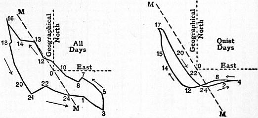
Fig. 9. Fig. 10.

In temperate latitudes the differences of type are much less, but still they exist. A good idea of their ordinary size and character in the case of declination may be derived from Table XXIX., containing data for Kew, Greenwich and Parc St Maur.

The data for Greenwich are due to W. Ellis30, those for Parc St Maur to T. Moureaux33. The quantity tabulated is the algebraic excess of the all or ordinary day mean hourly value over the corresponding quiet day value in the mean diurnal inequality for the year. At Greenwich and Kew days of extreme disturbance have been excluded from the ordinary days, but apparently not at Parc St Maur. The number of highly disturbed days at the three stations is, however, small, and their influence is not great. The differences disclosed by Table XXIX. are obviously of a systematic character, which would not tend to disappear however long a period was utilized. In short, while the diurnal inequality from quiet days may be that most truly representative of undisturbed conditions, it does not represent the average state of conditions at the station. To go into full details respecting the differences between all and quiet days would occupy undue space, so the following brief summary of the differences observed in declination at Kew must suffice. While the inequality range is but little different for the two types of days, the mean of the hourly differences from the mean for the day is considerably reduced in the quiet days. The 24-hour term in the Fourier analysis is of smaller amplitude in the quiet days, and its phase angle is on the average about 6°.75 smaller than on ordinary days, implying a retardation of about 27 minutes in the time of maximum. The diurnal inequality range is more variable throughout the year in quiet days than on ordinary days, and the same is true of the absolute ranges. The tendency to a secondary minimum in the range at midsummer is considerably more decided on ordinary than on quiet days. When the variation throughout the year in the diurnal inequality range is expressed in Fourier series, whose periods are the year and its submultiples, the 6-month term is notably larger for ordinary than for quiet days. Also the date of the maximum in the 12-month term is about three days earlier for ordinary than for quiet days. The exact size of the differences between ordinary and quiet day phenomena must depend to some extent on the criteria employed in selecting quiet days and in excluding disturbed days. This raises difficulties when it comes to comparing results at different stations. For stations near together the difficulty is trifling. The astronomer royal’s quiet days have been used for instance at Parc St. Maur, Val Joyeux, Falmouth and Kew, as well as at Greenwich. But when stations are wide apart there are two obvious difficulties: first, the difference of local time; secondly, the fact that a day may be typically quiet at one station but appreciably disturbed at the other.

If the typical quiet day were simply the antithesis of a disturbed day, it would be natural to regard the non-cyclic change on quiet days as a species of recoil from some effect of disturbance. This view derives support from the fact, pointed out long ago by Sabine34, that the horizontal force usually, though by no means always, is lowered by magnetic disturbances. Dr van Bemmelen35 who has examined non-cyclic phenomena at a number of stations, seems disposed to regard this as a sufficient explanation. There are, however, difficulties in accepting this view. Thus, whilst the non-cyclic effect in horizontal force and inclination at Kew and Falmouth appeared on the whole enhanced in years of sun-spot maximum, the difference between years such as 1892 and 1894 on the one hand, and 1890 and 1900 on the other, was by no means proportional to the excess of disturbance in the former years. Again, when the average non-cyclic change of declination was calculated at Kew for 207 days, selected as those of most marked irregular disturbance between 1890 and 1900, the sign actually proved to be the same as for the average quiet day of the period.

Table XXIX.—All or Ordinary, less Quiet Day Hourly Values (+ to the West).

Hour. Forenoon. Afternoon.

Kew 1890-1900. Greenwich 1890-1894. Parc St Maur 1883-1897. Kew 1890-1900. Greenwich 1890-1894. Parc St Maur 1893-1897.

′ ′ ′ ′ ′ ′

1 −0.58 −0.59 −0.63 +0.42 +0.44 +0.40

2 −0.54 −0.47 −0.47 +0.52 +0.45 +0.50

3 −0.51 −0.31 −0.32 +0.57 +0.52 +0.59

4 −0.41 −0.23 −0.16 +0.60 +0.51 +0.55

5 −0.28 −0.10 −0.01 +0.46 +0.34 +0.38

6 −0.08 +0.12 +0.18 +0.21 +0.04 +0.07

7 +0.13 +0.30 +0.34 −0.06 −0.24 −0.25

8 +0.29 +0.48 +0.47 −0.27 −0.50 −0.54

9 +0.40 +0.56 +0.53 −0.47 −0.68 −0.74

10 +0.44 +0.58 +0.51 −0.61 −0.78 −0.79

11 +0.48 +0.50 +0.44 −0.62 −0.77 −0.79

12 +0.45 +0.44 +0.38 −0.54 −0.61 −0.67

§ 31. A satisfactory definition of magnetic disturbance is about as difficult to lay down as one of heterodoxy. The idea in its generality seems to present no difficulty, but it is a very different matter when one comes to details. Amongst Magnetic Disturbances. the chief disturbances recorded since 1890 are those of February 13-14 and August 12, 1892; July 20 and August 20, 1894; March 15-16, and September 9, 1898; October 31, 1903; February 9-10, 1907; September 11-12, 1908 and September 25, 1909. On such days as these the oscillations shown by the magnetic curves are large and rapid, aurora is nearly always visible in temperate latitudes, earth currents are prominent, and there is interruption—sometimes very serious—in the transmission of telegraph messages both in overhead and underground wires. At the other end of the scale are days on which the magnetic curves show practically no movement beyond the slow regular progression of the regular diurnal inequality. But between these two extremes there are an infinite variety of intermediate cases. The first serious attempt at a precise definition of disturbance seems due to General Sabine35a. His method had once an extensive vogue, and still continues to be applied at some important observatories. Sabine regarded a particular observation as disturbed when it differed from the mean of the observations at that hour for the whole month by not less than a certain limiting value. His definition takes account only of the extent of the departure from the mean, whether the curve is smooth at the time or violently oscillating makes no difference. In dealing with a particular station Sabine laid down separate limiting values for each element. These limits were the same, irrespective of the season of the year or of the sun-spot frequency. A departure, for example, of 3′.3 at Kew from the mean value of declination for the hour constituted a disturbance, whether it occurred in December in a year of sun-spot minimum, or in June in a year of sun-spot maximum, though the regular diurnal inequality range might be four times as large in the second case as in the first. The limiting values varied from station to station, the size depending apparently on several considerations not very clearly defined. Sabine subdivided the disturbances in each element into two classes: the one tending to increase the element, the other tending to diminish it. He investigated how the numbers of the two classes varied throughout the day and from month to month. He also took account of the aggregate value of the disturbances of one sign, and traced the diurnal and annual variations in these aggregate values. He thus got two sets of diurnal variations and two sets of annual variations of disturbance, the one set depending only on the number of the disturbed hours, the other set considering only the aggregate value of the disturbances. Generally the two species of disturbance variations were on the whole fairly similar. The aggregates of the + and − disturbances for a particular hour of the day were seldom equal, and thus after the removal of the disturbed values the mean value of the element for that hour was generally altered. Sabine’s complete scheme supposed that after the criterion was first applied, the hourly means would be recalculated from the undisturbed values and the criterion applied again, and that this process would be repeated until the disturbed observations all differed by not less than the accepted limiting value from the final mean based on undisturbed values alone. If the disturbance limit were so small that the disturbed readings formed a considerable fraction of the whole number, the complete execution of Sabine’s scheme would be exceedingly laborious. As a matter of fact, his disturbed readings were usually of the order of 5% of the total number, and unless in the case of exceptionally large magnetic storms it is of little consequence whether the first choice of disturbed readings is accepted as final or is reconsidered in the light of the recalculated hourly means.

Sabine applied his method to the data obtained during the decade 1840 to 1850 at Toronto, St Helena, Cape of Good Hope and Hobart, also to data for Pekin, Nertchinsk, Point Barrow, Port Kennedy and Kew. C. Chambers36 applied it to data from Bombay. The yearly publication of the Batavia observatory gives corresponding results for that station, and Th. Moureaux 33 has published similar data for Parc St Maur. Tables XXX. to XXXII. are based on a selection of these data. Tables XXX. and XXXI. show the annual variation in Sabine’s disturbances, the monthly values being expressed as percentages of the arithmetic mean value for the 12 months. The Parc St Maur and Batavia data, owing to the long periods included, are especially noteworthy. Table XXX. deals with the east (E) and west (W) disturbances of declination separately. Table XXXI., dealing with disturbances in horizontal and vertical force, combines the + and − disturbances, treated numerically. At Parc St Maur the limits required to qualify for disturbance were 3′.0 in D, 20γ in H, and 12γ in V; the corresponding limits for Batavia were 1′.3, 11γ and 11γ. The limits for D at Toronto, Bombay and Hobart were respectively 3′.6, 1′.4 and 2′.4.

At Parc St Maur the disturbance data from all three elements give distinct maxima near the equinoxes; a minimum at midwinter is clearly shown, and also one at midsummer, at least in D and H. A decline in disturbance at midwinter is visible at all the stations, but at Batavia the equinoctial values for D and V are inferior to those at midsummer.

Table XXX.—Annual Variation of Disturbances (Sabine’s numbers).

Parc St Maur 1883-97. Toronto 1841-48. Bombay 1859-65. Batavia 1883-99. Hobart 1843-48.

Month. E. W. E. W. E. W. E. W. E. W.

January 78 60 55 66 89 89 180 223 165 182

February 116 92 75 86 94 67 138 144 121 116

March 126 107 92 94 129 97 102 87 114 104

April 105 113 115 114 106 129 67 73 110 102

May 101 118 101 101 63 99 72 71 62 53

June 77 89 95 72 78 81 45 27 32 37

July 82 104 140 126 121 173 62 46 50 49

August 88 113 137 133 154 131 69 69 86 78

September 134 137 163 139 111 108 135 144 135 114

October 119 115 101 111 140 128 95 88 124 123

November 99 94 73 85 43 43 106 91 79 111

December 75 58 51 72 72 55 124 137 123 130

Table XXXII. shows in some cases a most conspicuous diurnal variation in Sabine’s disturbances. The data are percentages of the totals for the whole 24 hours. But whilst at Batavia the easterly and westerly disturbances in D vary similarly, at Parc St Maur they follow opposite laws, the easterly showing a prominent maximum near noon, the westerly a still more prominent maximum near midnight. The figures in the second last line of the table, if divided by 0.24, will give the percentage of hours which show the species of disturbance indicated. For instance, at Parc St Maur, out of 100 hours, 3 show disturbances to the west and 3.7 to the east; or in all 6.7 show disturbances of declination. The last line gives the average size of a disturbance of each type, the unit being 1′ in D and 1γ in H and V.

Table XXXI.—Annual Variation of Disturbances.

Parc St Maur. Toronto. Batavia.

Month. Numbers. Aggregates. Numbers. Aggregates.

H. V. H. V. H. V. H. V.

January 81 51 58 56 96 151 89 154

February 96 133 94 74 105 123 110 125

March 126 118 94 108 116 105 117 103

April 94 111 150 149 104 76 105 73

May 108 133 90 112 101 92 105 95

June 90 85 36 50 82 69 79 66

July 99 128 61 71 90 83 95 81

August 113 92 75 108 91 91 98 91

September 119 122 171 160 113 111 114 115

October 101 94 148 129 114 89 104 86

November 104 81 98 75 99 102 100 101

December 70 51 128 100 89 108 84 110

At Batavia disturbances increasing and decreasing the element are about equally numerous, but this is exceptional. Easterly disturbances of declination predominated at Toronto, Point Barrow, Fort Kennedy, Kew, Parc St Maur, Bombay and the Falkland Islands whilst the reverse was true of St Helena, Cape of Good Hope, Pekin and Hobart. At Kew and Parc St Maur the ratios borne by the eastern to the western disturbances were 1.19 and 1.23 respectively, and so not much in excess of unity; but the preponderance of easterly disturbances at the North American37 stations was considerably larger than this.

Table XXXII.—Diurnal Variation of Disturbances (Sabine’s numbers).

Hour. Parc St Maur. Batavia.

D. H. V. D. H. V.

E. W. + − + − E. W. + − + −

0-3 10.1 20.3 9.0 8.3 5.7 9.2 1.1 5.8 13.1 6.6 4.0 7.4

3-6 12.3 8.2 8.4 8.0 6.4 10.4 7.6 7.3 14.2 4.8 6.3 10.0

6-9 15.7 3.8 14.1 12.5 7.2 9.0 24.9 16.8 12.1 9.9 21.2 21.7

9-noon 16.2 5.1 18.0 15.6 12.9 15.4 38.5 33.0 8.6 15.8 19.8 16.4

noon-3 19.3 6.7 15.3 16.5 18.2 18.3 18.8 24.7 16.8 21.1 23.5 22.1

3-6 14.8 9.7 12.5 15.4 22.9 21.8 6.4 5.4 13.3 16.9 12.6 12.7

6-9 5.7 21.2 11.4 13.2 18.9 11.2 2.3 3.4 9.9 13.6 7.1 4.1

9-12 5.9 25.0 11.2 10.5 7.8 4.7 0.4 3.8 12.0 11.1 5.6 5.4

Mean number per day 0.88 0.72 1.15 1.56 1.04 0.96 0.46 0.44 1.62 1.61 1.19 1.13

Mean size · · · · · · · · · · · · 1.72 1.69 18.0 19.5 16.7 15.5

§ 32. From the point of view of the surveyor there is a good deal to be said for Sabine’s definition of disturbance, but it is less satisfactory from other standpoints. One objection has been already indicated, viz. the arbitrariness of applying the same limiting value at a station irrespective of the size of the normal diurnal range at the time. Similarly it is arbitrary to apply the same limit between 10 a.m. and noon, when the regular diurnal variation is most rapid, as between 10 p.m. and midnight, when it is hardly appreciable. There seems a distinct difference of phase between the diurnal inequalities on different types of days at the same season; also the phase angles in the Fourier terms vary continuously throughout the year, and much more rapidly at some stations and at some seasons than at others. Thus there may be a variety of phenomena which one would hesitate to regard as disturbances which contribute to the annual and diurnal variations in Tables XXX. to XXXII.

Sabine, as we have seen, confined his attention to the departure of the hourly reading from the mean for that hour. Another and equally natural criterion is the apparent character of the magnetograph curve. At Potsdam curves are regarded as “1” quiet, “2” moderately disturbed, or “3” highly disturbed. Any hourly value to which the numeral 3 is attached is treated as disturbed, and the annual Potsdam publication contains tables giving the annual and diurnal variations in the number of such disturbed hours for D, H and V. According to this point of view, the extent to which the hourly value departs from the mean for that hour is immaterial to the results. It is the greater or less sinuosity and irregularity of the curve that counts. Tables XXXIII. and XXXIV. give an abstract of the mean Potsdam results from 1892 to 1901. The data are percentages: in Table XXXIII. of the mean monthly total, in Table XXXIV. of the total for the day. So far as the annual variation is concerned, the results in Table XXXIII. are fairly similar to those in Table XXX. for Parc St Maur. There are pronounced maxima near the equinoxes, especially the spring equinox. The diurnal variations, however, in Tables XXXII. and XXXIV. are dissimilar. Thus in the case of H the largest disturbance numbers at Parc St Maur occurred between 6 a.m. and 6 p.m., whereas in Table XXXIV. they occur between 4 p.m. and midnight. Considering the comparative proximity of Parc St Maur and Potsdam, one must conclude that the apparent differences between the results for these two stations are due almost entirely to the difference in the definition of disturbance.

Table XXXIII.—Annual Variation of Potsdam Disturbances.

Element. Jan. Feb. Mar. April. May. June. July. Aug. Sept. Oct. Nov. Dec.

D 129 170 149 90 86 57 62 64 59 118 94 82

H 109 133 131 102 109 82 94 91 89 101 75 84

V 106 171 170 108 121 56 64 74 93 87 78 70

Mean 115 158 150 100 105 65 73 76 94 102 82 79

Table XXXIV.—Diurnal Variation of Potsdam Disturbances.

Hours. 1-3. 4-6. 7-9. 10-noon. 1-3. 4-6. 7-9. 10-12.

D 14.9 11.1 8.0 5.2 5.7 13.1 22.5 19.5

H 10.5 8.4 8.0 8.5 11.3 17.6 19.2 16.5

V 13.5 9.7 5.7 4.7 8.5 17.2 21.5 19.2

Mean 13.0 9.7 7.2 6.1 8.5 16.0 21.1 18.4

Table XXXV.—Disturbed Day less ordinary Day Inequality (Unit 1′, + to West).

Hour. 1 2 3 4 5 6 7 8 9 10 11 12

a.m. −3.4 −2.6 −2.0 −0.3 +1.6 +1.9 +2.3 +2.0 +2.1 +2.0 +1.6 +1.8

p.m. +1.8 +2.2 +2.1 +1.7 +1.4 0.0 −1.3 −2.8 −3.5 −2.6 −3.5 −2.4

One difficulty in the Potsdam procedure is the maintenance of a uniform standard. Unless very frequent reference is made to the curves of some standard year there must be a tendency to enter under “3” in quiet years a number of hours which would be entered under “2” in a highly disturbed year. Still, such a source of uncertainty is unlikely to have much influence on the diurnal, or even on the annual, variation.

§ 33. A third method of investigating a diurnal period in disturbances is to form a diurnal inequality from disturbed days alone, and compare it with the corresponding inequalities from ordinary or from quiet days. Table XXXV. gives some declination data for Kew, the quantity tabulated being the algebraic excess of the disturbed day hourly value over that for the ordinary day in the mean diurnal inequality for the year, as based on the 11 years 1890 to 1900.

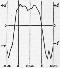
Fig. 11.

The disturbed day inequality was corrected for non-cyclic change in the usual way. Fig. 11 shows the results of Table XXXV. graphically. The irregularities are presumably due to the limited number, 209, of disturbed days employed; to get a smooth curve would require probably a considerably longer period of years. The differences between disturbed and ordinary days at Kew are of the same general character as those between ordinary and quiet days in Table XXIX.; they are, however, very much larger, the range in Table XXXV. being fully 5½ times that in Table XXIX. If quiet days had replaced ordinary days in Table XXXV., the algebraic excess of the disturbed day would have varied from +2′.7 at 2 p.m. to −4′.1 at 11 p.m., or a range of 6′.8.

§ 34. When the mean diurnal inequality in declination for the year at Kew is analysed into Fourier waves, the chief difference, it will be remembered, between ordinary and quiet days was that the amplitude of the 24-hour term was enhanced in the ordinary days, whilst its phase angle indicated an earlier occurrence of the maximum. Similarly, the chief difference between the Fourier waves for the disturbed and ordinary day inequalities at Kew is the increase in the amplitude of the 24-hour term in the former by over 70%, and the earlier occurrence of its maximum by about 1 hour 50 minutes. It is clear from these results for Kew, and it is also a necessary inference from the differences obtained by Sabine’s method between east and west or + and − disturbances, that there is present during disturbances some influence which affects the diurnal inequality in a regular systematic way, tending to make the value of the element higher during some hours and lower during others than it is on days relatively free from disturbance. At Kew the consequence is a notable increase in the range of the regular diurnal inequality on disturbed days; but whether this is the general rule or merely a local peculiarity is a subject for further research.

§ 35. There are still other ways of attacking the problem of disturbances. W. Ellis27 made a complete list of disturbed days at Greenwich from 1848 onwards, arranging them in classes according to the amplitude of the disturbance shown on the curves. Of the 18,000 days which he considered, Ellis regarded 2,119, or only about 12%, as undisturbed. On 11,898 days, or 66%, the disturbance movement in declination was under 10′; on 3614, or 20%, the disturbance, though exceeding 10′, was under 30′; on 294 days it lay between 30′ and 60′; while on 75 days it exceeded 60′. Taking each class of disturbances separately, Ellis found, except in the case of his “minor” disturbances—those under 10′—a distinct double annual period, with maxima towards the equinoxes. Subsequently C. W. Maunder,38 making use of these same data, and of subsequent data up to 1902, put at his disposal by Ellis, came to similar conclusions. Taking all the days with disturbances of declination over 10′, and dealing with 15-day periods, he found the maxima of frequency to occur the one a little before the spring equinox, the other apparently after the autumnal equinox; the two minima were found to occur early in June and in January. When the year is divided into three seasons—winter (November to February), summer (May to August), and equinox—Maunder’s figures lead to the results assigned to Greenwich disturbed days in Table XXXVI. The frequency in winter, it will be noticed, though less than at equinox, is considerably greater than in summer. This greater frequency in winter is only slightly apparent in the disturbances over 60′, but their number is so small that this may be accidental. The next figures in Table XXXVI. relate to highly disturbed days at Kew. The larger relative frequency at Kew in winter as compared to summer probably indicates no real difference from Greenwich, but is simply a matter of definition. The chief criterion at Kew for classifying the days was not so much the mere amplitude of the largest movement, as the general character of the day’s curve and its departure from the normal form. The data in Table XXXVI. as to magnetic storms at Greenwich are based on the lists given by Maunder39 in the Monthly Notices, R.A.S. A storm may last for any time from a few hours to several days, and during part of its duration the disturbance may not be very large; thus it does not necessarily follow that the frequencies of magnetic storms and of disturbed days will follow the same laws. The table shows, however, that so far as Greenwich is concerned the annual variations in the two cases are closely alike. In addition to mean data for the whole 56 years, 1848 to 1903, Table XXXVI. contains separate data for the 14 years of that period which represented the highest sun-spot frequency, and the 15 years which represented lowest sun-spot frequency. It will be seen that relatively considered the seasonal frequencies of disturbance are more nearly equal in the years of many than in those of few sun-spots. Storms are more numerous as a whole in the years of many sun-spots, and this preponderance is especially true of storms of the largest size. This requires to be borne in mind in any comparisons between larger and smaller storms selected promiscuously from a long period. An unduly large proportion of the larger storms will probably come from years of large sun-spot frequency, and there is thus a risk of assigning to differences between the laws obeyed by large and small storms phenomena that are due in whole or in part to differences between the laws followed in years of many and of few sun-spots. The last data in Table XXXVI. are based on statistics for Batavia given by W. van Bemmelen,40 who considers separately the storms which commence suddenly and those which do not. These sudden movements are recorded over large areas, sometimes probably all over the earth, if not absolutely simultaneously, at least too nearly so for differences in the time of occurrence to be shown by ordinary magnetographs. It is ordinarily supposed that these sudden movements, and the storms to which they serve as precursors, arise from some source extraneous to the earth, and that the commencement of the movement intimates the arrival, probably in the upper atmosphere, of some form of energy transmitted through space. In the storms which commence gradually the existence of a source external to the earth is not so prominently suggested, and it has been sometimes supposed that there is a fundamental difference between the two classes of storms. Table XXXVI. shows, however, no certain difference in the annual variation at Batavia. At the same time, this possesses much less significance than it would have if Batavia were a station like Greenwich, where the annual variation in magnetic storms is conspicuous.

Besides the annual period, there seems to be also a well-marked diurnal period in magnetic disturbances. This is apparent in Tables XXXVII. and XXXVIII., which contain some statistics for Batavia due to van Bemmelen, and some for Greenwich derived from the data in Maunder’s papers referred to above. Table XXXVII. gives the relative frequency of occurrence for two hour intervals, starting with midnight, treating separately the storms of gradual (g) and sudden (s) commencement. In Table XXXVIII. the day is subdivided into three equal parts. Batavia and Greenwich agree in showing maximum frequency of beginnings about the time of minimum frequency of endings and conversely; but the hours at which the respective maxima and minima occur at the two places differ rather notably.