VOLUME XVII SLICE III McKinley, William to Magnetism, Terrestrial (continued 10)

91 This deduction from Ewing’s theory appears to have been first suggested by J. Swinburne. See Industries, 1890, 289.

92 R. Beattie (Phil. Mag., 1901, 1, 642) has found similar effects in nickel and cobalt.

93 The charge associated with a corpuscle is the same as that carried by a hydrogen atom. G. J. Stoney in 1881 (Phil. Mag., 1881, 11, 387) pointed out that this latter constituted the indivisible “atom of electricity” or natural unit charge. Later he proposed (Trans. Roy. Dub. Soc., 1891, 4, 583) that such unit charge should be called an “electron.” The application of this term to Thomson’s corpuscle implies, rightly or wrongly, that notwithstanding its apparent mass, the corpuscle is in fact nothing more than an atom of electricity. The question whether a corpuscle actually has a material gravitating nucleus is undecided, but there are strong reasons for believing that its mass is entirely due to the electric charge.

94 Jour. de Phys., 1905, 4, 678; translated in Electrician, 1905, 56, 108 and 141.

95 The quotations are from the translation published by the Gilbert Club, London, 1900.

96 C. A. Coulomb, Mem. Acad. Roy. Paris, 1785, p. 578.

97 Intensitas vis magneticae, § 21, C. F. Gauss’s Werke, 5, 79. See also J. J. Thomson, Electricity and Magnetism, § 132.

98 S. D. Poisson, Mém. de l’Institut, 1821 and 1822, 5, 247, 488; 1823, 6, 441; 1838, 16, 479.

99 For outlines of the mathematical theory of magnetism and references see H. du Bois, Magnetic Circuit, chs. iii. and iv.

100 Gilbert’s Ann. d. phys., 1820, 6, 295.

101 Ann. de chim. et de phys., 1820, 15, 59, 170; Recueil d’observations électrodynamiques, 1822; Théories des phénomènes électrodynamiques, 1826.

102 Ann. de chim. et de phys., 1820, 15, 93.

103 Trans. Soc. Arts, 1825, 43, 38.

104 Phil. Mag., 1873, 46, 140; 1874, 48, 321.

105 Phil. Trans., 1885, 176, 523; Magnetic Induction, 1900.

106 Proc. Roy. Soc., 1890, 48, 342.

107 Phil. Mag., 1897, 44, 293; 1898, 46, 528.

MAGNETISM, TERRESTRIAL, the science which has for its province the study of the magnetic phenomena of the earth.

§ 1. Terrestrial magnetism has a long history. Its early growth was slow, and considerable uncertainty prevails as to its earliest developments. The properties of the magnet (see Magnetism) were to some small extent known to Historical. the Greeks and Romans before the Christian era, and compasses (see Compass) of an elementary character seem to have been employed in Europe at least as early as the 12th century. In China and Japan compasses of a kind seem to have existed at a much earlier date, and it is even claimed that the Chinese were aware of the declination of the compass needle from the true north before the end of the 11th century. Early scientific knowledge was usually, however, a mixture of facts, very imperfectly ascertained, with philosophical imaginings. When an early writer makes a statement which to a modern reader suggests a knowledge of the declination of the compass, he may have had no such definite idea in his mind. So far as Western civilization is concerned, Columbus is usually credited with the discovery—in 1492 during his first voyage to America—that the pointing of the compass needle to the true north represents an exceptional state of matters, and that a declination in general exists, varying from place to place. The credit of these discoveries is not, however, universally conceded to Columbus. G. Hellmann6A considers it almost certain that the departure of the needle from the true north was known in Europe before the time of Columbus. There is indirect evidence that the declination of the compass was not known in Europe in the early part of the 15th century, through the peculiarities shown by early maps believed to have been drawn solely by regard to the compass. Whether Columbus was the first to observe the declination or not, his date is at least approximately that of its discovery.

The next fundamental discovery is usually ascribed to Robert Norman, an English instrument maker. In The Newe Attractive (1581) Norman describes his discovery made some years before of the inclination or dip. The discovery was made more or less by accident, through Norman’s noticing that compass needles which were truly balanced so as to be horizontal when unmagnetized, ceased to be so after being stroked with a magnet. Norman devised a form of dip-circle, and found a value for the inclination in London which was at least not very wide of the mark.

Another fundamental discovery, that of the secular change of the declination, was made in England by Henry Gellibrand, professor of mathematics at Gresham College, who described it in his Discourse Mathematical on the Variation of the Magneticall Needle together with its Admirable Diminution lately discovered (1635). The history of this discovery affords a curious example of knowledge long delayed. William Borough, in his Discourse on the Variation of the Compas or Magneticall Needle (1581), gave for the declination at Limehouse in October 1580 the value 11°¼ E. approximately. Observations were repeated at Limehouse, Gellibrand tells us, in 1622 by his colleague Edmund Gunter, professor of astronomy at Gresham College, who found the much smaller value 6° 13′. The difference seems to have been ascribed at first to error on Borough’s part, and no suspicion of the truth seems to have been felt until 1633, when some rough observations gave a value still lower than that found by Gunter. It was not until midsummer 1634 that Gellibrand felt sure of his facts, and yet the change of declination since 1580 exceeded 7°. The delay probably arose from the strength of the preconceived idea, apparently universally held, that the declination was absolutely fixed. This idea, it would appear, derived some of its strength from the positive assertion made on the point by Gilbert of Colchester in his De magnete (1600).

A third fundamental discovery, that of the diurnal change in the declination, is usually credited to George Graham (1675-1751), a London instrument maker. Previous observers, e.g. Gellibrand, had obtained slightly different values for the declination at different hours of the day, but it was natural to assign them to instrumental uncertainties. In those days the usual declination instrument was the compass with pivoted needles, and Graham himself at first assigned the differences he observed to friction. The observations on which he based his conclusions were made in 1722; an account of them was communicated to the Royal Society and published in the Philosophical Transactions for 1724.

The movements of the compass needle throughout the average day represent partly a regular diurnal variation, and partly irregular changes in the declination. The distinction, however, was not at first very clearly realized. Between 1756 and 1759 J. Canton observed the declination-changes on some 600 days, and was thus able to deduce their general character. He found that the most prominent part of the regular diurnal change in England consisted of a westerly movement of the north-pointing pole from 8 or 9 a.m. to 1 or 2 p.m., followed by a more leisurely return movement to the east. He also found that the amplitude of the movement was considerably larger in summer than in winter. Canton further observed that in a few days the movements were conspicuously irregular, and that aurora was then visible. This association of magnetic disturbance and aurora had, however, been observed somewhat before this time, a description of one conspicuous instance being contributed to the Royal Society in 1750 by Pehr Vilhelm Wargentin (1717-1783), a Swede.

Another landmark in the history of terrestrial magnetism was the discovery towards the end of the 18th century that the intensity of the resultant magnetic force varies at different parts of the earth. The first observations clearly showing this seem to be those of a Frenchman, Paul de Lamanon, who observed in 1785-1787 at Teneriffe and Macao, but his results were not published at the time. The first published observations seem to be those made by the great traveller Humboldt in tropical America between 1798 and 1803. The delay in this discovery may again be attributed to instrumental imperfections. The method first devised for comparing the force at different places consisted in taking the time of oscillation of the dipping needle, and even with modern circles this is hardly a method of high precision. Another discovery worth chronicling was made by Arago in 1827. From observations made at Paris he found that the inclination of the dipping needle and the intensity of the horizontal component of the magnetic force both possessed a diurnal variation.

§ 2. Whilst Italy, England and France claim most of the early observational discoveries, Germany deserves a large share of credit for the great improvement in instruments and methods during the first half of the 19th century. Measurements of the intensity of the magnetic force were somewhat crude until Gauss showed how absolute results could be obtained, and not merely relative data based on observations with some particular needle. Gauss also devised the bifilar magnetometer, which is still largely represented in instruments measuring changes of the horizontal force; but much of the practical success attending the application of his ideas to instruments seems due to Johann von Lamont (1805-1879), a Jesuit of Scottish origin resident in Germany.

The institution of special observatories for magnetic work is largely due to Humboldt and Gauss. The latter’s observatory at Göttingen, where regular observations began in 1834, was the centre of the Magnetic Union founded by Gauss and Weber for the carrying out of simultaneous magnetic observations and it was long customary to employ Göttingen time in schemes of international co-operation.

In the next decade, mainly through the influence of Sir Edward Sabine (1788-1883), afterwards president of the Royal Society, several magnetic observatories were established in the British colonies, at St Helena, Cape of Good Hope, Hobarton (now Hobart) and Toronto. These, with the exception of Toronto, continued in full action for only a few years; but their records—from their widely distributed positions—threw much fresh light on the differences between magnetic phenomena in different regions of the globe. The introduction of regular magnetic observatories led ere long to the discovery that there are notable differences between the amplitudes of the regular daily changes and the frequency of magnetic disturbances in different years. The discovery that magnetic phenomena have a period closely similar to, if not absolutely identical with, the “eleven year” period in sun-spots, was made independently and nearly simultaneously about the middle of the 19th century by Lamont, Sabine and R. Wolf.

The last half of the 19th century showed a large increase in the number of observatories taking magnetic observations. After 1890 there was an increased interest in magnetic work. One of the contributory causes was the magnetic survey of the British Isles made by Sir A. Rücker and Sir T. E. Thorpe, which served as a stimulus to similar work elsewhere; another was the institution by L. A. Bauer of a magazine. Terrestrial Magnetism, specially devoted to the subject. This increased activity added largely to the stock of information, sometimes in forms of marked practical utility; it was also manifested in the publication of a number of papers of a speculative character. For historical details the writer is largely indebted to the works of E. Walker1 and L. A. Bauer.3

§ 3. All the more important magnetic observatories are provided with instruments of two kinds. Those of the first kind give the absolute value of the magnetic elements at the time of observation. The unifilar magnetometer (q.v.), for Observational Methods and Records. instance, gives the absolute values of the declination and horizontal force, whilst the inclinometer (q.v.) or dip circle gives the inclination of the dipping needle. Instruments of the second kind, termed magnetographs (q.v.), are differential and self-recording, and show the changes constantly taking place in the magnetic elements. The ordinary form of magnetograph records photographically. Light reflected from a fixed mirror gives a base line answering to a constant value of the element in question; the light is cut off every hour or second hour so that the base line also serves to make the time. Light reflected from a mirror carried by a magnet gives a curved line answering to the changes in position of the magnet. The length of the ordinate or perpendicular drawn from any point of the curved line on to the base line is proportional to the extent of departure of the magnet from a standard position. If then we know the absolute value of the element which corresponds to the base line, and the equivalent of 1 cm. of ordinate, we can deduce the absolute value of the element answering to any given instant of time. In the case of the declination the value of 1 cm. of ordinate is usually dependent almost entirely on the distance of the mirror carried by the magnet from the photographic paper, and so remains invariable or very nearly so. In the case of the horizontal force and vertical force magnetographs—these being the two force components usually recorded—the value of 1 cm. of ordinate alters with the strength of the magnet. It has thus to be determined from time to time by observing the deflection shown on the photographic paper when an auxiliary magnet of known moment, at a measured distance, deflects the magnetograph magnet. Means are provided for altering the sensitiveness, for instance, by changing the effective distance in the bifilar suspension of the horizontal force magnet, and by altering the height of a small weight carried by the vertical force magnet. It is customary to aim at keeping the sensitiveness as constant as possible. A very common standard is to have 1 cm. of ordinate corresponding to 10′ of arc in the declination and to 50γ (1γ ≡ 0.00001 C.G.S.) in the horizontal and vertical force magnetographs.

As an example of how the curves are standardized, suppose that absolute observations of declination are taken four times a month, and that in a given month the mean of the observed values is 16° 34′.6 W. The curves are measured at the places which correspond to the times of the four observations, and the mean length of the four ordinates is, let us say, 2.52 cms. If 1 cm. answers to 10′, then 2.52 cms. represents 25′.2, and thus the value of the base line—i.e. the value which the declination would have if the curve came down to the base line—is for the month in question 16° 34′.6 less 25′.2 or 16° 9′.4. If now we wish to know the declination at any instant in this particular month all we have to do is to measure the corresponding ordinate and add its value, at the rate of 10′ per cm., to the base value 16° 9′.4 just found. Matters are a little more complicated in the case of the horizontal and vertical force magnetographs. Both instruments usually possess a sensible temperature coefficient, i.e. the position of the magnet is dependent to some extent on the temperature it happens to possess, and allowance has thus to be made for the difference from a standard temperature. In the case of the vertical force an “observed” value is derived by combining the observed value of the inclination with the simultaneous value of the horizontal force derived from the horizontal force magnetograph after the base value of the latter has been determined. In themselves the results of the absolute observations are of minor interest. Their main importance is that they provide the means of fixing the value of the base line in the curves. Unless they are made carefully and sufficiently often the information derivable from the curves suffers in accuracy, especially that relating to the secular change. It is from the curves that information is derived as to the regular diurnal variation and irregular changes. In some observatories it is customary to publish a complete record of the values of the magnetic elements at every hour for each day of the year. A useful and not unusual addition to this is a statement of the absolutely largest and smallest values of each element recorded during each day, with the precise times of their occurrence. On days of large disturbance even hourly readings give but a very imperfect idea of the phenomena, and it is customary at some observatories, e.g. Greenwich, to reproduce the more disturbed curves in the annual volume. In calculating the regular diurnal variation it is usual to consider each month separately. So far as is known at present, it is entirely or almost entirely a matter of accident at what precise hours specially high or low values of an element may present themselves during an individual highly disturbed day; whilst the range of the element on such a day may be 5, 10 or even 20 times as large as on the average undisturbed day of the month. It is thus customary when calculating diurnal inequalities to omit the days of largest disturbance, as their inclusion would introduce too large an element of uncertainty. Highly disturbed days are more than usually common in some years, and in some months of the year, thus their omission may produce effects other than that intended. Even on days of lesser disturbance difficulties present themselves. There may be to and fro movements of considerable amplitude occupying under an hour, and the hour may come exactly at the crest or at the very lowest part of the trough. Thus, if the reading represents in every case the ordinate at the precise hour a considerable element of chance may be introduced. If one is dealing with a mean from several hundred days such “accidents” can be trusted to practically neutralize one another, but this is much less fully the case when the period is as short as a month. To meet this difficulty it is customary at some observatories to derive hourly values from a freehand curve of continuous curvature, drawn so as to smooth out the apparently irregular movements. Instead of drawing a freehand curve it has been proposed to use a planimeter, and to accept as the hourly value of the ordinate the mean derived from a consideration of the area included between the curve, the base line and ordinates at the thirty minutes before and after each hour.

§ 4. Partly on account of the uncertainties due to disturbances, and partly with a view to economy of labour, it has been the practice at some observatories to derive diurnal inequalities from a comparatively small number of undisturbed or quiet days. Beginning with 1890, five days a month were selected at Greenwich by the astronomer royal as conspicuously quiet. In the selection regard was paid to the desirability that the arithmetic mean of the five dates should answer to near the middle of the month. In some of the other English observatories the routine measurement of the curves was limited to these selected quiet days. At Greenwich itself diurnal inequalities were derived regularly from the quiet days alone and also from all the days of the month, excluding those of large disturbance. If a quiet day differed from an ordinary day only in that the diurnal variation in the latter was partly obscured by irregular disturbances, then supposing enough days taken to smooth out irregularities, one would get the same diurnal inequality from ordinary and from quiet days. It was found, however, that this was hardly ever the case (see §§ 29 and 30). The quiet day scheme thus failed to secure exactly what was originally aimed at; on the other hand, it led to the discovery of a number of interesting results calculated to throw valuable sidelights on the phenomena of terrestrial magnetism.

The idea of selecting quiet days seems due originally to H. Wild. His selected quiet days for St Petersburg and Pavlovsk were very few in number, in some months not even a single day reaching his standard of freedom from disturbance. In later years the International Magnetic Committee requested the authorities of each observatory to arrange the days of each month in three groups representing the quiet, the moderately disturbed and the highly disturbed. The statistics are collected and published on behalf of the committee, the first to undertake the duty being M. Snellen. The days are in all cases counted from Greenwich midnight, so that the results are strictly synchronous. The results promise to be of much interest.

§ 5. The intensity and direction of the resultant magnetic force at a spot—i.e. the force experienced by a unit magnetic pole—are known if we know the three components of force parallel to any set of orthogonal axes. It is usual to take for these axes the vertical at the spot and two perpendicular axes in the horizontal plane; the latter are usually taken in and perpendicular to the geographical meridian. The usual notation in mathematical work is X to the north, Y to the west or east, and Z vertically downwards. The international magnetic committee have recommended that Y be taken positive to the east, but the fact that the declination is westerly over most of Europe has often led to the opposite procedure, and writers are not always as careful as they should be in stating their choice. Apart from mathematical calculations, the more usual course is to define the force by its horizontal and vertical components—usually termed H and V—and by the declination or angle which the horizontal component makes with the astronomical meridian. The declination is sometimes counted from 0° to 360°, 0° answering to the case when the so-called north pole (or north seeking pole) is directed towards geographical north, 90° to the case when it is directed to the east, and so on. It is more usual, however, to reckon declination only from 0° to 180°, characterizing it as easterly or westerly according as the north pole points to the east or to the west of the geographical meridian. The force is also completely defined by H or V, together with D the declination, and I the inclination to the horizon of the dipping needle. Instead of H and D some writers make use of N the northerly component, and W the westerly (or E the easterly). The resultant force itself is denoted sometimes by R, sometimes by T (total force). The following relationships exist between the symbols

X ≡ N, Y ≡ W or E, Z ≡ V, R ≡ T, H ≡ √(X² + Y²), R ≡ √(X² + Y² + Z²), tan D = Y / X, tan I = V / H.

The term magnetic element is applied to R or any of the components, and even to the angles D and I.

§ 6. Declination is the element concerning which our knowledge is most complete and most reliable. With a good unifilar magnetometer, at a fixed observatory distant from the magnetic poles, having a fixed mark of Charts. known azimuth, the observational uncertainty in a single observation should not exceed 0′.5 or at most 1′.0. It cannot be taken for granted that different unifilars, even by the best makers, will give absolutely identical values for the declination, but as a matter of fact the differences observed are usually very trifling. The chief source of uncertainty in the observation lies in the torsion of the suspension fibre, usually of silk or more rarely of phosphor bronze or other metal. A very stout suspension must be avoided at all cost, but the fibre must not be so thin as to have a considerable risk of breaking even in skilled hands. Near a magnetic pole the directive force on the declination magnet is reduced, and the effects of torsion are correspondingly increased. On the other hand, the regular and irregular changes of declination are much enhanced. If an observation consisting of four readings of declination occupies twelve minutes, the chances are that in this time the range at an English station will not exceed 1′, whereas at an arctic or antarctic station it will frequently exceed 10′. Much greater uncertainty thus attaches to declination results in the Arctic and Antarctic than to those in temperate latitudes. In the case of secular change data one important consideration is that the observations should be taken at an absolutely fixed spot, free from any artificial source of disturbance. In the case of many of the older observations of which records exist, the precise spot cannot be very exactly fixed, and not infrequently the site has become unsuitable through the erection of buildings not free from iron. Apart from buildings, much depends on whether the neighbourhood is free from basaltic and other magnetic rocks. If there are no local disturbances of this sort, a few yards difference is usually without appreciable influence, and even a few miles difference is of minor importance when one is calculating the mean secular change for a long period of years. When, however, local disturbances exist, even a few feet difference in the site may be important, and in the absence of positive knowledge to the contrary it is only prudent to act as if the site were disturbed. Near a magnetic pole the declination naturally changes very rapidly when one travels in the direction perpendicular to the lines of equal declination, so that the exact position of the site of observation is there of special importance.

The usual method of conveying information as to the value of the declination at different parts of the earth’s surface is to draw curves on a map—the so-called isogonals—such that at all points on any one curve the declination at a given specified epoch has the same value. The information being of special use to sailors, the preparation of magnetic charts has been largely the work of naval authorities—more especially of the hydrographic department of the British admiralty. The object of the admiralty world charts—four of which are reproduced here, on a reduced scale, by the kind permission of the Hydrographer—is rather to show the general features boldly than to indicate minute details. Apart from the immediate necessities of the case, this is a counsel of prudence. The observations used have mostly been taken at dates considerably anterior to that to which the chart is intended to apply. What the sailor wants is the declination now or for the next few years, not what it was five, ten or twenty years ago. Reliable secular change data, for reasons already indicated, are mainly obtainable from fixed observatories, and there are enormous areas outside of Europe where no such observatories exist. Again, as we shall see presently, the rate of the secular change sometimes alters greatly in the course of a comparatively few years. Thus, even when the observations themselves are thoroughly reliable, the prognostication made for a future date by even the most experienced of chart makers may be occasionally somewhat wide of the mark. Fig. 1 is a reduced copy of the British admiralty declination chart for the epoch 1907. It shows the isogonals between 70° N. and 65° S. latitude. Beyond the limits of this chart, the number of exact measurements of declination is somewhat limited, but the general nature of the phenomena is easily inferred. The geographical and the magnetic poles—where the dipping needle is vertical—are fundamental points. The north magnetic pole is situated in North America near the edge of the chart. We have no reason to suppose that the magnetic pole is really a fixed point, but for our present purpose we may regard it as such. Let us draw an imaginary circle round it, and let us travel round the circle in the direction, west, north, east, south, starting from a point where the north pole of a magnet (i.e. the pole which in Europe or the United States points to the north) is directed exactly towards the astronomical north. The point we start from is to the geographical south of the magnetic pole. As we go round the circle the needle keeps directed to the magnetic pole, and so points first slightly to the east of geographical north, then more and more to the east, then directly east, then to south of east, then to due south, to west of south, to west, to north-west, and finally when we get round to our original position due north once more. Thus, during our course round the circle the needle will have pointed in all possible directions. In other words, isogonals answering to all possible values of the declination have their origin in the north magnetic pole. The same remark applies of course to the south magnetic pole.

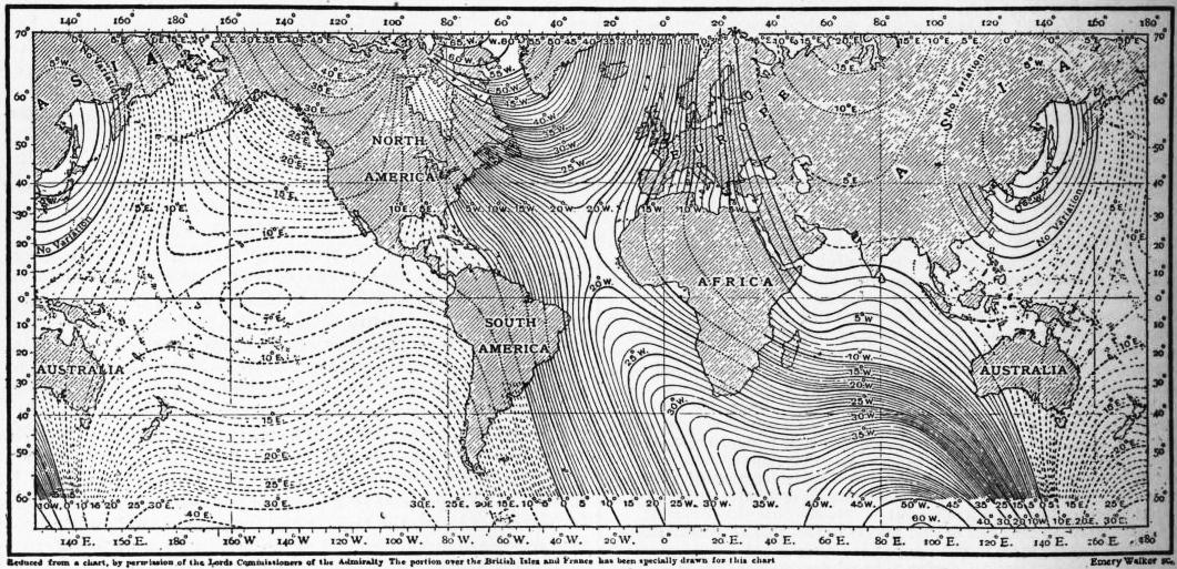
Fig. 1.—Isogonals, or lines of equal magnetic declination.

Now, suppose ourselves at the north geographical pole of the earth. Neglecting as before diurnal variation and similar temporary changes, and assuming no abnormal local disturbance, the compass needle at and very close to this pole will occupy a fixed direction relative to the ground underneath. Let us draw on the ground through the pole a straight line parallel to the direction taken there by the compass needle, and let us carry a compass needle round a small circle whose centre is the pole. At all points on the circle the positions of the needle will be parallel; but whereas the north pole of the magnet will point exactly towards the centre of the circle at one of the points where the straight line drawn on the ground cuts the circumference, it will at the opposite end of the diameter point exactly away from the centre. The former part is clearly on the isogonal where the declination is 0°, the latter on the isogonal where it is 180°. Isogonals will thus radiate out from the north geographical pole (and similarly of course from the south geographical pole) in all directions. If we travel along an isogonal, starting from the north magnetic pole, our course will generally take us, often very circuitously, to the north geographical pole. If, for example, we select the isogonal of 10° E., we at first travel nearly south, but then more and more westerly, then north-westerly across the north-east of Asia; the direction then gets less northerly, and makes a dip to the south before finally making for the north geographical pole. It is possible, however, according to the chart, to travel direct from the north magnetic to the south geographical pole, provided we select an isogonal answering to a small westerly or easterly declination (from about 19° W. to 7° E.).

Special interest attaches to the isogonals answering to declination 0°. These are termed agonic lines, but sailors often call them lines of no variation, the term variation having at one time been in common use in the sense of declination. If we start from the north magnetic pole the agonic line takes us across Canada, the United States and South America in a fairly straight course to the south geographical pole. A curve continuous with this can be drawn from the south geographical to the south magnetic pole at every point of which the needle points in the geographical meridian; but here the north pole of the needle is pointing south, not north, so that this portion of curve is really an isogonal of 180°. In continuation of this there emanates from the south magnetic pole a second isogonal of 0°, or agonic line, which traverses Australia, Arabia and Russia, and takes us to the north geographical pole. Finally, we have an isogonal of 180°, continuous with this second isogonal of 0° which takes us to the north magnetic pole, from which we started. Throughout the whole area included within these isogonals of 0° and 180°—excluding locally disturbed areas—the declination is westerly; outside this area the declination is in general easterly. There is, however, as shown in the chart, an isogonal of 0° enclosing an area in eastern Asia inside which the declination is westerly though small.

§ 7. Fig. 2 is a reduced copy of the admiralty chart of inclination or dip for the epoch 1907. The places where the dip has the same value lie on curves called isoclinals. The dip is northerly (north pole dips) or southerly (south pole dips) according as the place is north or south of the isoclinal of 0°. At places actually on this isoclinal the dipping needle is horizontal. The isoclinal of 0° is nowhere very far from the geographical equator, but lies to the north of it in Asia and Africa, and to the south of it in South America. As we travel north from the isoclinal of 0° along the meridian containing the magnetic pole the dipping needle’s north pole dips more and more, until when we reach the magnetic pole the needle is vertical. Going still farther north, we have the dip diminishing. The northerly inclination is considerably less in Europe than in the same latitudes of North America; and correspondingly the southerly inclination is less in South America than in the same latitudes of Africa.

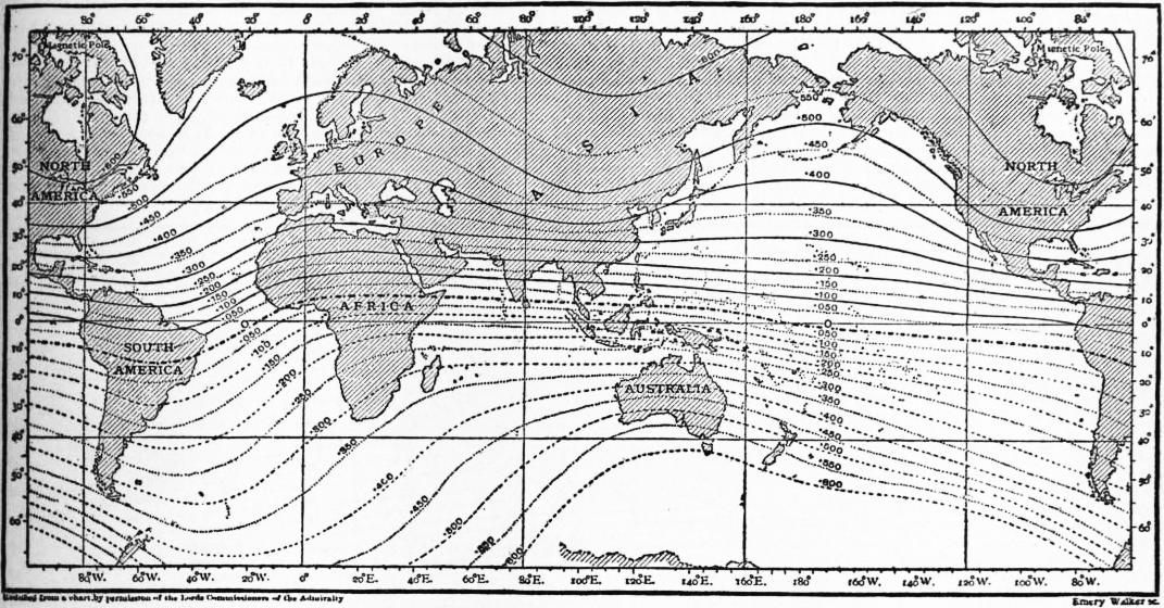
Fig. 2.—Isoclinals, or lines of equal magnetic dip.

Fig. 3 is a reduced copy of the admiralty horizontal force chart for 1907. The curves, called isomagnetics, connect the places where the horizontal force has the same value; the force is expressed in C.G.S. units. The horizontal force vanishes of course at the magnetic poles. The chart shows a maximum value of between 0.39 and 0.40 in an oval including the south of Siam and the China Sea. The horizontal force is smaller in North America than in corresponding latitudes in Europe.

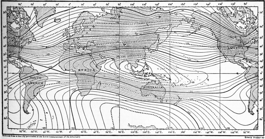
Fig. 3.—Isomagnetics, lines of equal horizontal force.

Charts are sometimes drawn for other magnetic elements, especially vertical force (fig. 4) and total force. The isomagnetic of zero vertical force coincides necessarily with that of zero dip, and there is in general considerable resemblance between the forms of lines of equal vertical force and those of equal dip. The highest values of the vertical force occur in areas surrounding the magnetic poles, and are fully 50% larger than the largest values of the horizontal force. The total force is least in equatorial regions, where values slightly under 0.4 C.G.S. are encountered. In the northern hemisphere there are two distinct maxima of total force. One of these so-called foci is in Canada, the other in the north-east of Siberia, the former having the higher value of the force. There are, however, higher values of the total force than at either of these foci throughout a considerable area to the south of Australia. In the northern hemisphere the lines of equal total force—called isodynamic lines—form two sets more or less distinct, consisting of closed ovals, one set surrounding the Canadian the other the Siberian focus.

§ 8. As already explained, magnetic charts for the world or for large areas give only a general idea of the values of the elements. If the region is undisturbed, very fairly approximate values are derivable from the charts, but when the highest accuracy is necessary Magnetic Elements and their Secular Change. the only thing to do is to observe at the precise spot. In disturbed areas local values often depart somewhat widely from what one would infer from the chart, and occasionally there are large differences between places only a few miles apart. Magnetic observatories usually publish the mean value for the year of their magnetic elements. It has been customary for many years to collect and publish these results in the annual report of the Kew Observatory (Observatory Department of the National Physical Laboratory). The data in Tables I. and II. are mainly derived from this source. The observatories are arranged in order of latitude, and their geographical co-ordinates are given in Table II., longitude being reckoned from Greenwich. Table I. gives the mean values of the declination, inclination and horizontal force for January 1, 1901; they are in the main arithmetic means of the mean annual values for the two years 1900 and 1901. The mean annual secular changes given in this table are derived from a short period of years—usually 1898 to 1903—the centre of which fell at the beginning of 1901. Table II. is similar to Table I., but includes vertical force results; it is more extensive and contains more recent data. In it the number of years is specified from which the mean secular change is derived; in all cases the last year of the period employed was that to which the absolute values assigned to the element belong. The great majority of the stations have declination west and inclination north; it has thus been convenient to attach the + sign to increasing westerly (or decreasing easterly) declination and to increasing northerly (or decreasing southerly) inclination. In other words, in the case of the declination + means that the north end of the needle is moving to the west, while in the case of the inclination + means that the north end (whether the dipping end or not) is moving towards the nadir. In the case, however, of the vertical force + means simply numerical increase, irrespective of whether the north or the south pole dips. The unit employed in the horizontal and vertical force secular changes is 1γ, i.e. 0.00001 C.G.S. Even in the declination, at the very best observatories, it is hardly safe to assume that the apparent change from one year to the next is absolutely truthful to nature. This is especially the case if there has been any change of instrument or observer, or if any alteration has been made to buildings in the immediate vicinity. A change of instrument is a much greater source of uncertainty in the case of horizontal force or dip than in the case of declination, and dip circles and needles are more liable to deterioration than magnetometers. Thus, secular change data for inclination and vertical force are the least reliable. The uncertainties, of course, are much less, from a purely mathematical standpoint, for secular changes representing a mean from five or ten years than for those derived from successive years’ values of the elements. The longer, however, the period of years, the greater is the chance that one of the elements may in the course of it have passed through a maximum or minimum value. This possibility should always be borne in mind in cases where a mean secular change appears exceptionally small.

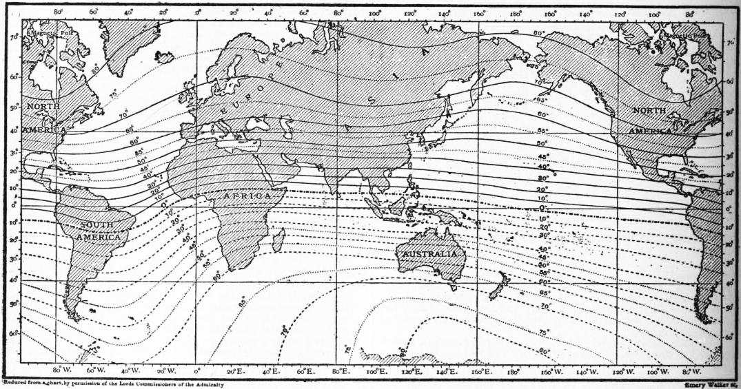
Fig. 4.—Isomagnetics, lines of equal vertical force.

As Tables I. and II. show, the declination needle is moving to the east all over Europe, and the rate at which it is moving seems not to vary much throughout the continent. The needle is also moving to the east throughout the western parts of Asia, the north and east of Africa, and the east of North America. It is moving to the west in the west of North America, in South America, and in the south and east of Asia, including Japan, south-east Siberia, eastern China and most of India.

§ 9. The information in figs. 1, 2, 3 and 4 and in Tables I. and II. applies only to recent years. Owing to secular change, recent charts differ widely from the earliest ones constructed. The first charts believed to have been constructed were those of Edmund Halley the astronomer. According to L. A. Bauer,7 who has made a special study of the subject, Halley issued two declination charts for the epoch 1700; one, published in 1701, was practically confined to the Atlantic Ocean, whilst the second, published in 1702, contained also data for the Indian Ocean and part of the Pacific. These charts showed the isogonic lines, but only over the ocean areas. Though the charts for 1700 were the first published, there are others which apply to earlier epochs. W. van Bemmelen8 has published charts for the epochs 1500, 1550, 1600, 1650 and 1700, whilst H. Fritsche9 has more recently published charts of declination, inclination and horizontal force for 1600, 1700, 1780, 1842 and 1915. A number of early declination charts were given in Hansteen’s Atlas and in G. Hellmann’s reprints. Die Altesten Karten der Isogonen, Isoklinen, Isodynamen (Berlin, 1895). The data for the earlier epochs, especially those prior to 1700, are meagre, and in many cases probably of indifferent accuracy, so that the reliability of the charts for these epochs is somewhat open to doubt.

If we take either Hansteen’s or Fritsche’s declination chart for 1600 we notice a profound difference from fig. 1. In 1600 the agonic line starting from the north magnetic pole, after finding its way south to the Gulf of Mexico, doubled back to the north-east, and passed across or near Iceland. After getting well to the north of Iceland it doubled again to the south, passing to the east of the Baltic. The second agonic line which now lies to the west of St Petersburg appears in 1600 to have continued, after traversing Australia, in a nearly northerly direction through the extreme east of China. The nature of the changes in declination in western Europe will be understood from Table III., the data from which, though derived from a variety of places in the south-east of England,10 may be regarded as approximately true of London. The earliest result is that obtained by Borough at Limehouse. Those made in the 16th century are due to Gunter, Gellibrand, Henry Bond and Halley. The observations from 1787 to 1805 were due to George Gilpin, who published particulars of his own and the earlier observations in the Phil. Trans. for 1806. The data for 1817 and 1820 were obtained by Col. Mark Beaufoy, at Bushey, Herts. They seem to come precisely at the time when the needle, which had been continuously moving to the west since the earliest observations, began to retrace its steps. The data from 1860 onwards apply to Kew.

Table I.—Magnetic Elements and their Rate of Secular Change for January 1, 1901.

Place. Absolute values. Secular change.

D. I. H. D. I. H.

° ′ ° ′ ′ ′ γ

Pavlovsk 0 39.8E 70 36.8N .16553 − 4.1 −0.8 + 7

Ekatarinburg 10 6.3E 70 40.5N .17783 − 4.6 +0.5 −13

Copenhagen 10 10.4W 68 38.5N .17525

Stonyhurst 18 10.3W 68 48.0N .17330 − 4.0 +22

Wilhelmshaven 12 26.0W 67 39.7N .18108 − 4.1 −2.1 +20

Potsdam 9 54.2W 66 24.5N .18852 − 4.2 −1.6 +16

Irkutsk 2 1.0E 70 15.8N .20122 + 0.5 +1.6 −14

de Bilt 13 48.3W 66 55.5N .18516 − 4.4 −2.2 +14

Kew 16 50.8W 67 10.6N .18440 − 4.2 −2.2 +25

Greenwich 16 27.5W 67 7.3N .18465 − 4.0 −2.2 +23

Uccle 14 11.0W 66 8.8N .18954 − 4.2 −2.1 +23

Falmouth 18 27.3W 66 44.0N .18705 − 3.8 −2.7 +26

Prague 9 4.4W .19956 − 4.4 +20 +20

St Helier 16 58.1W 65 44.1N − 3.5 −2.7

Parc St Maur 14 43.4W 64 52.3N .19755 − 4.0 −2.2 +23

Val Joyeux 15 13.7W 65 0.0N .19670

Munich 10 25.8W 63 18.1N .20629 − 4.8 −2.7 +21

O’Gyalla 7 26.1W .21164 − 4.8 +13

Pola 9 22.7W 60 14.5N .22216 − 4.0 +23

Toulouse 14 16.4W 60 55.9N .21945 − 3.9 −2.5 +25

Perpignan 13 34.7W 59 57.6N .22453

Capo di Monte 9 8.0W 56 22.3N − 5.2 −2.3

Madrid 15 39.0W

Coimbra 17 18.1W 59 22.0N .22786 − 3.7 −4.3 +34

Lisbon 17 15.7W 57 53.0N .23548

Athens 5 38.2W 52 7.5N .26076

San Fernando 15 57.5W 55 8.8N .24648

Tokyo 4 34.9W 49 0.3N .29932

Zi−ka−wei 2 23.5W 45 43.5N .32875 + 1.5 −1.5 +37

Helwan 3 39.7W 40 30.8N .30136 − 7.0 −0.4 − 7

Hong−Kong 0 17.5E 31 22.8N .36753 + 1.8 −4.3 +45

Kolaba 0 23.2E 21 26.5N .37436 + 2.2 +7.0 − 9

Manila 0 52.2E 16 13.5N .38064 + 0.1 −5.3 +47

Batavia 1 7.3E 30 35.5S .36724 + 3.0 −7.3 −11

Mauritius 9 25.2W 54 9.4S .23820 − 4.7 +4.6 −39

Rio de Janeiro 8 2.9W 13 20.1S .2501 +10.4 −2.3

Melbourne 8 25.6E 67 24.6S .23295

The rate of movement of the needle to the east at London—and throughout Europe generally—fell off markedly subsequent to 1880. The change of declination in fact between 1880 and 1895 was only about 75% of that between 1865 and 1880, and the mean annual change from 1895 to 1900 was less than 75% of the mean annual change of the preceding fifteen years. Thus in 1902 it was at least open to doubt whether a change in the sign of the secular change were not in immediate prospect. Subsequent, however, to that date there was little further decline in the rate of secular change, and since 1905 there has been very distinct acceleration. Thus, if we derive a mean value from the eighteen European stations for which declination secular changes are given in Tables I. and II. we find

mean value from table I. −4.18

” ” ” ” II. −5.21

The epoch to which the data in Table II. refer is somewhat variable, but is in all cases more recent than the epoch, January 1, 1901, for Table I., the mean difference being about 5 years.

§ 10. At Paris there seems to have been a maximum of easterly declination (about 9°) about 1580; the needle pointed to true north about 1662, and reached its extreme westerly position between 1812 and 1814. The phenomena at Rome resembled those at Paris and London, but the extreme westerly position is believed to have been attained earlier. The rate of change near the turning point seems to have been very slow, and as no fixed observatories existed in those days, the precise time of its occurrence is open to some doubt.

Perhaps the most complete observations extant as to the declination phenomena near a turning point relate to Kolaba observatory at Bombay; they were given originally by N. A. F. Moos,11 the director of the observatory. Some of the more interesting details are given in Table IV.; here W denotes movement to be west, and so answers to a numerical diminution in the declination, which is easterly.

Prior to 1880 the secular change at Kolaba was unmistakably to the east, and subsequent to 1883 it was clearly to the west; but between these dates opinions will probably differ as to what actually happened. The fluctuations then apparent in the sign of the annual change may be real, but it is at least conceivable that they are of instrumental origin. From 1870 to 1875 the mean annual change was −1′.2; from 1885 to 1890 it was +1′.5, from 1890 to 1895 it was +2′.0, while from 1895 to 1905 it was +2′.35, the + sign denoting movement to the west. Thus, in this case the rate of secular change has increased fairly steadily since the turning point was reached.

Table V. contains some data for St Helena and the Cape of Good Hope,12 both places having a long magnetic history. The remarkable feature at St Helena is the uniformity in the rate of secular change. The figures for the Cape show a reversal in the direction of the secular change about 1840, but after a few years the arrested movement to the west again became visible. According, however, to J. C. Beattie’s Magnetic Survey of South Africa the movement to the west ceased shortly after 1870. A persistent movement to the east then set in, the mean annual change increasing from 1′.8 between 1873 and 1890 to 3′.8 between 1890 and 1900.

§ 11. Secular changes of declination have been particularly interesting in the United States, an area about which information is unusually complete, thanks to the labours and publications of the United States Coast and Geodetic Survey.13 At present the agonic line passes in a south-easterly direction from Lake Superior to South Carolina. To the east of the agonic line the declination is westerly, and to the west it is easterly. In 1905 the declination varied from about 21° W. in the extreme north-east to about 24° E. in the extreme north-west. At present the motion of the agonic line seems to be towards the west, but it is very slow. To the east of the agonic line westerly declination is increasing, and to the west of the line, with the exception of a narrow strip immediately adjacent to it, easterly declination is increasing. The phenomena in short suggest a motion southwards in the north magnetic pole. Since 1750 declination has always been westerly in the extreme east of the States, and always easterly in the extreme west, but the position of the agonic line has altered a good deal. It was to the west of Richmond, Virginia, from 1750 to about 1772, then to the east of it until about 1838 when it once more passed to the west; since that time it has travelled farther to the west. Table VI. is intended to show the nature of the secular change throughout the whole country. As before, + denotes that the north pole of the magnet is moving to the west,—that it is moving to the east.

The data in Table VI. represent the mean change of declination per annum, derived from the period (ten years, except for 1900-1905) which ended in the year put at the top of the column. The stations are arranged in four groups, the first group representing the extreme eastern, the last group the extreme western states, the other two groups being intermediate. In each group the stations are arranged, at least approximately, in order of latitude. The data are derived from the values of the declination given in the Geodetic Survey’s Report for 1906, appendix 4, and Magnetic Tables and Magnetic Charts by L. A. Bauer, 1908. The values seem, in most cases, based to some extent on calculation, and very probably the secular change was not in reality quite so regular as the figures suggest. For the Western States the earliest data are comparatively recent, but for some of the eastern states data earlier than any in the table appear in the Report of the Coast and Geodetic Survey for 1902. These data indicate that the easterly movement of the magnet, visible in all the earlier figures for the Eastern States in Table VI., existed in all of them at least as far back as 1700. There is not very much evidence as to the secular change between 1700 and 1650, the earliest date to which the Coast and Geodetic Survey’s figures refer. The figures show a maximum of westerly declination about 1670 in New Jersey and about 1675 in Maryland. They suggest that this maximum was experienced all along the Atlantic border some time in the 17th century, but earlier in the extreme north-east than in New York or Maryland.

Examination of Table VI. shows that the needle continued to move to the east for some time after 1750 even in the Eastern States. But the rate of movement was clearly diminishing, and about 1765 the extreme easterly position was reached in Eastport, Maine, the needle then beginning to retrace its steps to the west. The phenomena visible at Maine are seen repeating themselves at places more and more to the west, in Boston about 1785, in Albany about 1800, in Washington, D.C., about 1805, in Columbus (Ohio) about 1815, in Montgomery (Alabama) about 1825, in Bloomington (Ill.) about 1830, in Des Moines (Iowa) about 1840, in Santa Rosa (New Mexico) about 1860 and in Salt Lake about 1870. In 1885 the needle was moving to the west over the whole United States with the exception of a comparatively narrow strip along the Pacific coast. Even an acute observer would have been tempted to prophesy in 1885 that at no distant date the secular change would be pronouncedly westerly right up to the Pacific. But in a few years a complete change took place. The movement to the east, which had become exceedingly small, if existent, in the Pacific states, began to accelerate; the movement to the west continued in the central, as in the eastern states, but perceptibly slackened. In 1905 the area throughout which the movement to the west still continued had greatly contracted and lay to the east of a line drawn from the west end of Lake Superior to the west of Georgia. If we take a station like Little Rock (Arkansas), we have the secular change to the west lasting for about sixty years. Further west the period shortens. At Pueblo (Colorado) it is about forty years, at Salt Lake under thirty years, at Prescott (Arizona) about twenty years. Considering how fast the area throughout which the secular change is easterly has extended to the east since 1885, one would be tempted to infer that at no distant date it will include the whole of the United States. In the extreme north-east, however, the movement of the needle to the west, which had slackened perceptibly after 1860 or 1870, is once more accelerating. Thus the auspices do not all point one way, and the future is as uncertain as it is interesting.

Table II.—Recent Values of the Magnetic Elements and their Rate of Secular Change.

Place. Geographical position. Absolute Values of Elements. Secular change (mean per annum).

Latitude. Longitude. Year. D. I. H. V. Interval in years. D. I. H. V.

° ′ ° ′ ° ′ ° ′ ′ ′

Pavlovsk 59 41N 30 29E 1906 1 4.2E 70 36.6N .16528 .46963 5 −4.5 +0.1 − 6 −14

Sitka (Alaska) 57 3N 135 20W 1906 30 3.3E 74 41.7N .15502 .56646 4 −3.0 −1.6 +18 −38

Ekatarinburg 56 49N 60 38E 1906 10 31.0E 70 49.5N .17664 .50796 5 −4.5 +1.7 −23 +18

Rude Skov (Copenhagen) 55 51N 12 27E 1908 9 43.3W 68 45N .17406 .44759

Stonyhurst 53 51N 2 28W 1909 17 28.6W 68 42.8N .17424 .44722 5 −5.9 −1.1 + 6 −25

Hamburg 53 33N 9 59E 1903 11 10.2W 67 23.5N .18126 .43527

Wilhelmshaven 53 32N 8 9E 1909 11 46.8W .18129 5 −5.2 − 7

Potsdam 52 23N 13 4E 1909 9 10.6W 66 20.0N .18834 .42971 5 −5.8 +0.1 − 9 −19

Irkutsk 52 16N 104 16E 1905 1 58.1E 70 25.0N .20011 .56250 5 +0.6 +2.0 −24 +39

de Bilt 52 5N 5 11E 1907 13 19.0W 66 49.9N .18559 .43368 5 −4.7 −0.6 + 2 −16

Valencia 51 56N 10 15W 1909 20 50.3W 68 15.1N .17877 .44812 5 −5.0 −1.2 + 7 −25

Kew 51 28N 0 19W 1909 16 10.8W 66 59.7N .18506 .43588 5 −5.4 −1.1 + 2 −35

Greenwich 51 28N 0 0 1909 15 47.6W 66 53.9N .18526 .43432 5 −5.5 −0.7 + 1 −20

Uccle 50 48N 4 21E 1908 13 36.7W 66 1.6N .19061 .42867 4 −5.3 −0.8 − 3 −35

Falmouth 50 9N 5 5W 1909 17 48.4W 66 30.6N .18802 .43266 5 −4.7 −1.4 + 9 −30

Prague 50 5N 14 25E 1908 8 20.9W 5 −6.5

Cracow 50 4N 19 58E 1909 5 35.1W 64 18N 3 −7.3

St Helier 49 12N 2 5W 1907 16 27.4W 65 34.5N 5 −5.3 −1.2

Val Joyeux 48 49N 2 1E 1909 14 32.9W 64 43.9N .19727 .41792 5 −5.4 −1.7 + 1 −51

Vienna 48 15N 16 21E 1898 8 24.1W

Munich 48 9N 11 37E 1906 9 59.5W 63 10.0N .20657 .40835 5 −4.8 −1.3 + 4 −31

O’Gyalla 47 53N 18 12E 1909 6 43.9W .21094 5 −5.0 −10

Odessa 46 26N 30 46E 1899 4 36.7W 62 18.2N .21869 .41660

Pola 44 52N 15 51E 1908 8 43.2W 60 6.8N .22207 .38640 5 −5.5 −0.6 − 4 −23

Agincourt (Toronto) 43 47N 79 16W 1906 5 45.3W 74 35.6N .16397 .59502 4 +3.4 +0.9 −23 −24

Nice 43 43N 7 16E 1899 12 4.0W 60 11.7N .22390 .39087

Toulouse 43 37N 1 28E 1905 13 56.3W 60 49.1N .22025 .39439 5 −4.5 −1.5 + 2 − 2

Perpignan 42 42N 2 53E 1907 13 4.4W 7 −4.7

Tiflis 41 43N 44 48E 1905 2 41.6E 56 2.8N .25451 .37799 7 −5.2 +1.7 −26 + 2

Capo di Monte 40 52N 14 15E 1906 8 40.3W 56 13.5N 5 −5.1 −1.5

Madrid 40 25N 3 40W 1901 15 35.6W

Coimbra 40 12N 8 25W 1908 16 46.2W 58 57.3N .22946 .38120 5 −4.6 −2.9 +17 −45

Baldwin (Kansas) 38 47N 95 10W 1906 8 30.1E 68 45.1N .21807 .56081 4 −1.7 +1.8 −36 − 8

Cheltenham(Maryland) 38 44N 76 50W 1906 5 22.0W 70 27.3N .20035 .56436 4 +3.8 +1.2 −38 −45

Lisbon 38 43N 9 9W 1900 17 18.0W 57 54.8N .23516 .37484

Athens 37 58N 21 23E 1908 4 52.9W 52 11.7N .26197 .33613 5 −5.5

San Fernando 36 28N 6 12W 1908 15 25.6W 54 48.4N .24829 .35206 5 −4.6 −2.8 +26 −24

Tokyo 35 41N 139 45E 1901 4 36.1W 49 0.0N .29954 .34459

Zi-ka-wei 31 12N 121 26E 1906 2 32.0W 45 35.3N .33040 .33726 5 +1.5 −1.3 +30 + 6

Dehra Dun 30 19N 78 3E 1907 2 38.3E 43 36.1N .33324 .31736 4 +0.8 +5.5 −26 +77

Helwan 29 52N 31 21E 1909 2 49.2W 40 40.4N .30031 .25804 5 −5.7 +1.2 − 6 +13

Havana 23 8N 82 25W 1905 2 25.0E 52 57.4N .30531 .40452

Barrackpore 22 46N 88 22E 1907 1 9.9E 30 30.2N .37288 .21967 3 +4.2 +3.4 +21 +62

Hong-Kong 22 18N 114 10E 1908 0 3.9E 31 2.5N .37047 .22292 5 +1.9 −1.8 +43 − 1

Honolulu 21 19N 158 4W 1906 9 21.7E 40 1.8N .29220 .24545 4 −0.9 −3.2 −19 −62

Kolaba 18 54N 72 49E 1905 0 14.0E 21 58.5N .37382 .15084 5 +2.1 +7.2 −11 +86

Alibagh 18 39N 72 52E 1909 1 0.3E 23 29.0N .36845 .16008 3 +1.7 +6.8 −10 +82

Vieques (Porto Rico) 18 9N 65 26W 1906 1 33.2W 49 47.7N .28927 .34224 2 +7.2 +6.8 −49 +66

Manila 14 35N 120 59E 1904 0 51.4E 16 0.2N .38215 .10960 5 +0.1 −3.9 +47 −34

Kodaikanal 10 14N 77 28E 1907 0 40.7W 3 27.2N .37431 .02259 4 +4.3 +5.5 +16 +61

Batavia 6 11S 106 49E 1906 0 54.1E 30 48.5S .36708 .21889 4 +2.1 −7.7 − 2 +110

Dar es Salaam 6 49S 39 18E 1903 7 35.2W

Mauritius 20 6S 57 33E 1908 9 14.3W 53 44.9S .23415 .31932 5 −0.3 +2.9 −53 −131

Rio de Janeiro 22 55S 43 11W 1906 8 55.5W 13 57.1S .24772 .06164 5 +9.1 −6.8 −42 +44

Santiago (Chile) 33 27S 70 42W 1906 14 18.7E 30 11.8S 3 +6.1 +9.9

Melbourne 37 50S 144 58E 1901 8 26.7E 67 25.0S .23305 .56024

Christchurch, N.Z. 43 32S 172 37E 1903 16 18.4E 67 42.3S .22657 .55259

Table III.—Declination at London.

Date. Declination. Date. Declination. Date. Declination.

° ′ ° ′ ° ′

1580 11 15E 1773 21 9W 1860 21 38.9W

1622 6 0 1787 23 19 1865 20 58.7

1634 4 6 1795 23 57 1870 20 18.3

1657 0 0 1802 24 6 1875 19 35.6

1665 1 22W 1805 24 8 1880 18 52.1

1672 2 30 1817 24 36 1885 18 19.2

1692 6 0 1818 24 38 1890 17 50.6

1723 14 17 1819 24 36 1895 17 16.8

1748 17 40 1820 24 34 1900 16 52.7

1905 16 32.9

§ 12. Table VII. gives particulars of the secular change of horizontal force and northerly inclination at London. Prior to the middle of the 19th century information as to the value of H is of uncertain value. The earlier inclination data14 are due to Norman, Gilbert, Bond, Graham, Heberden and Gilpin. The data from 1857 onwards, both for H and I, refer to Kew. “London” is rather a vague term, but the differences between the values of H and I at Kew and Greenwich—in the extreme west and east—are almost nil. For some time after its discovery by Robert Norman inclination at London increased. The earlier observations are not sufficient to admit of the date of the maximum inclination or its absolute value being determined with precision. Probably the date was near 1723. This view is supported by the fact that at Paris the inclination fell from 72° 15′ in 1754 to 71° 48′ in 1780. The earlier observations in London were probably of no very high accuracy, and the rates of secular change deducible from them are correspondingly uncertain. It is not improbable that the average annual change 0′.8 derived from the thirteen years 1773-1786 is too small, and the value 6′.2 derived from the fifteen years 1786-1801 too large. There is, however, other evidence of unusually rapid secular change of inclination towards the end of the 18th century in western Europe; for observations in Paris show a fall of 56′ between 1780 and 1791, and of 90′ between 1791 and 1806. Between 1801 and 1901 inclination in London diminished by 3° 26′.5, or on the average by 2′.1 per annum, while between 1857 and 1900 H increased on the average by 22γ a year. These values differ but little from the secular changes given in Table I. as applying at Kew for the epoch Jan. 1, 1901. Since the beginning, however, of the 20th century a notable change has set in, which seems shared by the whole of western Europe. This is shown in a striking fashion by contrasting the data from European stations in Tables I. and II. There are fifteen of these stations which give secular change data for H in both tables, while thirteen give secular data for I. The mean values of the secular changes derived from these stations are as follows:—

I H

From Table I. −2′.35 +21.0γ

From Table II. −1.12 +1.6γ

The difference in epoch between the two sets of results is only about 5 years, and yet in that short time the mean rate of annual increase in H fell to a thirteenth of its original value. During 1908-1909 H diminished throughout all Europe except in the extreme west. Whether we have to do with merely a temporary phase, or whether a general and persistent diminution in the value of H is about to set in over Europe it is yet hardly possible to say.

Table IV.—Declination at Kolaba (Bombay).

Year. Declination East. Change since previous year. Year. Declination East. Change since previous year.

° ′ ″ ′ ″ ° ′ ″ ′ ″

1876 0 55 58 0 37 E 1881 0 57 12 0 3 E

1877 56 39 0 41 E 1882 0 56 50 0 22 W

1878 57 6 0 27 E 1883 57 2 0 12 E

1879 57 30 0 24 E 1884 55 39 1 23 W

1880 57 9 0 21 W 1885 55 3 0 36 W

§ 13. It is often convenient to obtain a formula to express the mean annual change of an element during a given period throughout an area of some size. The usual method is to assume that the change at a place whose latitude is l and longitude λ is given by an expression of the type c + a(l − l0) + b(λ − λ0), where a, b, c are constants, l0 and λ0, denoting some fixed latitude and longitude which it is convenient to take as point of departure. Supposing observational data available from a series of stations throughout the area, a, b and c can be determined by least squares. As an example, we may take the following slightly modified formula given by Ad. Schmidt15 as applicable to Northern Europe for the period 1890 to 1900. ΔD, ΔI and ΔH represent the mean annual changes during this period in westerly declination, in inclination and in horizontal force:—

′ ′ ′

ΔD = −5.24 − 0.071 (l − 50) + 0.033 (λ − 10),

ΔI = −1.58 + 0.010 (l − 50) + 0.036 (λ − 10),

ΔH = +23.5 − 0.59 (l − 50) − 0.35 (λ − 10).

Longitude λ is here counted positive to the east. The central position assumed here (lat. 50°, long. 10° E.) falls in the north of Bavaria. In the case of the horizontal force unity represents 1γ. Schmidt found the above formulae to give results in very close agreement with the data at the eight stations which he had employed in determining the constants. These stations ranged from Pavlovsk to Perpignan, and from Stonyhurst to Ekaterinburg in Siberia. Formulae involving the second as well as the first powers of l − l0 and λ − λ0 have also been used, e.g., by A. Tanakadate in the Magnetic Survey of Japan.

Table V.—Declination at St Helena and Cape of Good Hope.

St Helena. Cape of Good Hope.

Date. Declination. Date. Declination.

° ′ ° ′

1610 7 13 E 1605 0 30 E

1677 0 40 1609 0 12 W

1691 1 0 W 1675 8 14

1724 7 30 1691 11 0

1775 12 18 1775 21 14

1789 15 30 1792 24 31

1796 15 48 1818 26 31

1806 17 18 1839 29 9

1839 22 17 1842 29 6

1840 22 53 1846 29 9

1846 23 11 1850 29 19

1890 23 57 1857 29 34

1874 30 4

1890 29 32

1903 28 44

Table VI.—Secular Change of Declination in the United States (+ to the West).

Place. Epoch 1760 70 80 90 1800 10 20 30 40 50 60 70 80 90 1900 50

′ ′ ′ ′ ′ ′ ′ ′ ′ ′ ′ ′ ′ ′ ′ ′

Eastport, Maine −1.2 0.0 +1.2 +2.1 +3.2 +4.0 +4.5 +4.9 +5.0 +5.6 +4.5 +3.0 +2.1 +1.0 +1.8 +2.4

Boston, Mass. −2.7 −1.9 −1.0 0.0 +1.1 +1.9 +2.7 +3.5 +4.2 +4.4 +4.0 +3.3 +3.1 +3.0 +3.2 +3.4

Albany, New York −4.2 −3.6 −2.7 −1.6 −0.6 +0.6 +1.6 +2.7 +3.6 +4.6 +4.6 +3.9 +4.7 +2.3 +3.4 +3.6

Philadelphia, Penn. −4.6 −4.2 −3.5 −2.3 −1.3 +0.1 +1.3 +2.5 +3.4 +4.3 +4.2 +4.6 +4.4 +3.4 +3.5 +3.4

Baltimore, Maryland −3.9 −3.4 −2.7 −2.0 −0.9 0.0 +0.9 +2.0 +2.7 +3.4 +3.9 +4.0 +3.9 +3.6 +3.5 +3.2

Richmond, Virginia −3.6 −3.2 −2.5 −1.8 −0.9 0.0 +0.9 +1.8 +2.5 +3.1 +3.6 +3.9 +3.8 +3.7 +3.4 +3.2

Columbia, S. Carolina −3.7 −3.4 −2.9 −2.2 −1.3 −0.5 +0.5 +1.3 +2.2 +2.9 +3.4 +3.8 +3.8 +3.8 +3.6 +1.8

Macon, Georgia −3.7 −3.6 −3.2 −2.5 −1.8 −0.9 0.0 +0.9 +1.8 +2.5 +3.2 +3.6 +3.9 +3.5 +3.1 +1.2

Tampa, Florida −3.0 −2.5 −2.0 −1.1 −0.4 +0.4 +1.1 +2.0 +2.5 +3.0 +3.2 +3.5 +3.7 +2.8 +2.9 +1.6

Marquette, Michigan 0.0 +1.4 +2.6 +3.7 +4.7 +5.1 +4.9 +3.8 +2.4

Columbus, Ohio −0.9 0.0 +0.9 +2.0 +2.9 +3.4 +3.6 +3.7 +3.9 +4.0 +2.4

Bloomington, Illinois −2.4 −1.5 −0.4 +0.4 +1.5 +2.4 +2.8 +4.2 +3.9 +2.9 +1.0

Lexington, Kentucky −0.9 0.0 +0.9 +1.8 +2.5 +3.2 +3.6 +3.8 +3.8 +3.4 +1.8

Chattanooga, Tennessee −0.9 0.0 +0.9 +1.8 +2.5 +3.2 +3.6 +4.0 +3.5 +3.1 +1.6

Little Rock, Arkansas −2.3 −1.5 −0.9 +0.1 +0.8 +1.7 +2.0 +3.6 +3.7 +2.3 −1.2

Montgomery, Alabama −3.6 −3.5 −3.1 −2.8 −2.2 −1.5 −0.8 +0.1 +0.8 +1.6 +2.2 +2.8 +3.8 +3.9 +2.6 +0.2

Alexandria, Louisiana −2.1 −1.6 −0.8 +0.1 +0.8 +1.6 +2.2 +3.6 +3.3 +2.0 −1.4

Northome, Minnesota −1.7 −0.6 +0.6 +1.7 +2.8 +4.2 +4.4 +3.5 0.0

Jamestown, N. Dakota +1.0 +1.9 +3.1 +4.8 +1.9 −2.2

Des Moines, Iowa −1.5 −0.6 +0.6 +1.5 +2.5 +3.8 +4.5 +2.7 −0.6

Douglas, Wyoming −0.8 0.0 +1.2 +2.3 +0.5 −1.6

Emporia, Kansas +0.6 +1.6 +2.7 +3.8 +1.7 −1.8

Pueblo, Colorado −0.3 +0.4 +1.5 +3.1 +0.7 −2.2

Okmulgee, Oklahoma +0.9 +1.5 +2.7 +3.9 +1.4 −2.4

Santa Rosa, New Mexico −0.4 +0.4 +1.4 +2.6 +0.4 −2.4

San Antonio, Texas −1.1 −0.5 −0.5 +1.1 +1.8 +2.7 +0.9 −2.4

Seattle, Washington −3.3 −3.5 −3.7 −3.7 −3.5 −3.3 −3.0 −2.6 −2.1 −1.3 −1.9 −2.0 −3.2

Wilson Creek, Washington −2.1 −1.5 −0.4 −1.0 −1.6 −3.2

Detroit, Oregon −3.8 −3.9 −3.9 −3.7 −3.4 −2.9 −2.5 −1.8 −0.8 −1.8 −3.8

Salt Lake, Utah −1.1 −0.4 +1.0 +1.0 −0.8 −2.8

Prescott, Arizona −1.4 −0.7 +0.4 +0.4 −1.2 −3.2

San José, California −2.6 −2.9 −2.9 −2.9 −2.7 −2.5 −2.3 −2.0 −1.5 −0.8 −0.4 −1.9 −3.8

Los Angeles, ” −3.4 −3.4 −3.5 −3.2 −3.0 −2.7 −2.1 −1.6 −1.1 −0.9 −0.3 −1.6 −3.6

Formulae are also wanted to show how the value of an element, or the rate of change of an element, at a particular place has varied throughout a long period. For comparatively short periods it is best to use formulae of the type E = a + bt + ct², where E denotes the value of an element t years subsequent to some convenient epoch; a, b, c are constants to be determined from the observational data. For longer periods formulae of the type E = a + b sin (mt + n), where a, b, m and n are constants, have been used by Schott16 and others with considerable success. The following examples, due to G. W. Littlehales,17 for the Cape of Good Hope, will suffice for illustration:

Declination (West) = 14°.63 + 15°.00 sin {0.61 (t − 1850) + 77°.8}.

Inclination (South) = 49°.11 + 8°.75 sin {0.8 (t − 1850) + 34°.3}.

Here t denotes the date. It is perhaps hardly necessary to point out that the extension of any of these empirical formulae—whether to places outside the surveyed area, or to times not included in the period of observation—is fraught with danger, which increases rapidly the further the extrapolation is pushed.

Table VII.—Inclination (northerly) and Horizontal Force at London.

Date. I. Date. I. Date. I. H. Date. I. H.

° ′ ° ′ ° ′ ° ′

1576 71 50 1801 70 36.0 1857 68 24.9 .17474 1891 67 33.2 .18193

1600 72 0 1821 70 3.4 1860 69 19.8 .17550 1895 67 25.4 .18278

1676 73 30 1830 69 38.0 1865 68 8.7 .17662 1900 67 11.8 .18428

1723 74 42 1838 69 17.3 1870 67 58.6 .17791 1905 67 3.8 .18510

1773 72 19 1854 68 31.1 1874 67 50.0 .17903 1908 67 0.9 .18515

1786 72 9

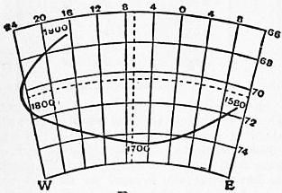
Fig. 5.

Bauer has employed a convenient graphical method of illustrating secular change. Radii are drawn from the centre of a sphere parallel to the direction of the freely dipping needle, and are produced to intersect the tangent plane drawn at the point which answers to the mean position of the needle during the epoch under consideration. The curve formed by the points of intersection shows the character of the secular change. Fig. 5 (slightly modified from Nature, vol. 57, p. 181) applies to London. The curve is being described in the clockwise direction. This, according to Bauer’s18 own investigation, is the normal mode of description. Schott and Littlehales have found, however, a considerable number of cases where it is difficult to say whether the motion is clockwise or not, while in some stations on both the east and west shores of the Pacific it was clearly anti-clockwise. Fritsche19 dealing with the secular changes from 1600 to 1885—as given by his calculated values of the magnetic elements—at 204 points of intersection of equidistant lines of latitude and longitude, found only sixty-three cases in which the motion was unmistakably clockwise, while in twenty-one cases it was clearly the opposite.

§ 14. All the magnetic elements at any ordinary station show a regular variation in the solar day. To separate this from the irregular changes, means of the hourly readings must be formed making use of a number of days. The amplitude of Diurnal Variations. the diurnal change usually varies considerably with the season of the year. Thus a diurnal inequality derived from all the days of the year combined, or from a smaller number of days selected equally from all the months of the year, can give only the average effect throughout the year. Also unless the hours of maxima and minima at a given station are but slightly variable with the season, the result obtained by combining data from all the months of the year may be a hybrid which does not very closely resemble the phenomena in the majority of individual months. This remark applies in particular to the declination at places within the tropics. One consequence is obviously to make the range of a diurnal inequality which answers to the year as a whole less than the arithmetic mean of the twelve ranges obtained for the constituent months. At stations in temperate latitudes, whilst minor differences of type do exist between the diurnal inequalities for different months of the year, the difference is mainly one of amplitude, and the mean diurnal inequality from all the months of the year gives a very fair idea of the nature of the phenomena in any individual month.

Table VIII.—Diurnal Inequality of Declination, mean from whole year (+ to West).

Station. Jan Mayen. St Petersburg and Pavlovsk. Greenwich. Kew. Parc St Maur. Tiflis. Kolaba. Batavia. Mauritius. South Vic- toria Land.

Latitude. 71° 0′ N. 59° 41′ N. 51° 28′ N. 51° 28′ N. 48° 49′ N. 41° 43′ N. 18° 54′ N. 6° 11′ S. 20° 6′ S. 77° 51′ S.

Longitude. 8° 28′ W. 30° 29′ E. 0° 0′. 0° 19′ W. 2° 29′ E. 44° 48′ E. 72° 49′ E. 106° 49′ E. 57° 33′ E. 166° 45′ E.

Period. 1882-1883. 1873-1885. 1890-1900. 1890-1900. 1883-1897. 1888-1898. 1894-1901. 1883-1894. 1876-1890. 1902-1903.

a. q. a. q. a. a. q. a. a. q. a. a. a. q.

Hour. ′ ′ ′ ′ ′ ′ ′ ′ ′ ′ ′ ′ ′ ′

1 − 6.6 −4.2 −1.3 −0.7 −1.4 −1.5 −0.9 −1.4 −0.7 −0.2 +0.1 +0.1 + 2.0 + 0.9

2 −10.5 −6.4 −1.2 −0.8 −1.3 −1.4 −0.9 −1.2 −0.6 −0.1 −0.1 +0.1 − 2.1 − 1.8

3 −15.2 −7.8 −1.2 −1.0 −1.3 −1.5 −1.0 −1.2 −0.6 −0.1 −0.1 +0.1 − 5.2 − 4.5

4 −16.9 −8.4 −1.4 −1.3 −1.4 −1.7 −1.3 −1.2 −0.5 −0.1 0.0 +0.2 − 9.4 − 6.8

5 −17.0 −8.1 −1.7 −1.8 −1.7 −2.1 −1.8 −1.6 −0.7 −0.1 0.0 +0.3 −12.2 − 9.0

6 −13.7 −7.0 −1.9 −2.3 −2.1 −2.4 −2.3 −1.9 −1.2 −0.6 +0.1 +0.4 −15.3 −11.7

7 − 9.3 −5.1 −2.2 −2.8 −2.4 −2.7 −2.8 −2.4 −1.9 −1.0 +0.5 +0.6 −17.2 −15.0

8 − 6.8 −3.2 −2.5 −3.2 −2.5 −2.8 −3.1 −2.7 −2.4 −1.2 +1.3 +1.1 −21.5 −17.3

9 − 3.7 −0.6 −2.3 −3.0 −1.9 −2.1 −2.5 −2.3 −2.3 −0.7 +1.7 +1.8 −23.5 −18.1

10 − 2.4 +2.1 −1.0 −1.7 −0.2 −0.3 −0.7 −0.5 −0.9 0.0 +1.5 +1.9 −21.2 −15.8

11 − 0.5 +4.6 +1.0 +0.4 +2.1 +2.2 +1.7 +2.0 +1.0 +0.9 +0.9 +1.3 −15.3 − 9.2

Noon + 2.5 +6.5 +3.1 +2.7 +4.2 +4.3 +3.9 +4.2 +2.6 +1.4 +0.1 0.0 − 9.8 − 4.9

1 + 3.7 +7.3 +4.6 +4.3 +5.1 +5.3 +4.8 +5.3 +3.3 +1.2 −0.6 −1.1 − 3.2 − 0.1

2 + 6.4 +7.1 +4.9 +4.5 +4.7 +4.9 +4.4 +4.9 +3.1 +0.6 −1.1 −2.0 + 3.8 + 5.9

3 + 7.4 +5.9 +4.1 +3.6 +3.6 +3.7 +3.1 +3.7 +2.3 +0.1 −1.3 −2.3 +11.1 + 9.5

4 + 8.5 +4.3 +2.7 +2.3 +2.2 +2.4 +1.8 +2.3 +1.3 −0.2 −1.2 −1.8 +16.6 +12.9

5 +10.6 +3.0 +1.5 +1.3 +1.1 +1.2 +0.7 +1.1 +0.6 −0.1 −0.9 −0.9 +19.9 +14.6

6 +14.2 +2.3 +0.6 +0.7 +0.3 +0.4 +0.2 +0.2 +0.2 0.0 −0.6 −0.1 +22.0 +15.5

7 +15.2 +2.2 0.0 +0.4 −0.3 −0.2 −0.1 −0.4 +0.1 +0.1 −0.4 +0.1 +22.0 +15.9

8 +15.8 +2.6 −0.4 +0.2 −0.9 −0.6 −0.3 −0.9 −0.1 +0.2 −0.2 +0.1 +19.9 +14.6

9 +13.2 +2.6 −1.0 0.0 −1.2 −1.0 −0.5 −1.3 −0.4 +0.1 0.0 +0.1 +16.0 +10.6

10 + 7.4 +2.0 −1.4 −0.2 −1.5 −1.3 −0.7 −1.5 −0.6 0.0 +0.1 +0.1 +11.6 + 7.2

11 + 1.1 +0.5 −1.6 −0.4 −1.6 −1.4 −0.8 −1.6 −0.7 0.0 +0.1 +0.1 + 7.6 + 4.2

12 − 3.6 −1.8 −1.5 −0.6 −1.6 −1.5 −0.9 −1.6 −0.8 −0.1 +0.1 +0.1 + 3.3 + 1.9

Range 32.8 15.7 7.4 7.7 7.6 8.1 7.9 8.0 5.7 2.6 3.0 4.2 45.5 34.0

Tables VIII. to XI. give mean diurnal inequalities derived from all the months of the year combined, the figures representing the algebraic excess of the hourly value over the mean for the twenty-four hours. The + sign denotes in Table VIII. that the north end of the needle is to the west of its mean position for the day; in Tables IX. to XI. it denotes that the element—the dip being the north or south as indicated—is numerically in excess of the twenty-four hour mean. The letter “a” denotes that all days have been included except, as a rule, those characterized by specially large disturbances. The letter “q” denotes that the results are derived from a limited number of days selected as being specially quiet, i.e. free from disturbance. In all cases the aperiodic or non-cyclic element—indicated by a difference between the values found for the first and second midnights of the day—has been eliminated in the usual way, i.e. by treating it as accumulating at a uniform rate throughout the twenty-four hours. The years from which the data were derived are indicated. The algebraically greatest and least of the hourly values are printed in heavy type; the range thence derived is given at the foot of the tables.

Table IX.—Diurnal Inequality of Horizontal Force, mean from whole year (Unit 1γ = .00001 C.G.S.)

Station. Jan Mayen. St Petersburg and Pavlovsk. Greenwich. Kew. Parc St Maur. Tiflis. Kolaba. Batavia. Mauritius. S. Victoria Land.

Period. 1882-1883. 1873-1885. 1890-1900. 1890-1900. 1883-1897. 1888-1898. 1894-1901. 1883-1894. 1883-1890. 1902-1903.

a. q. a. q. a. q. a. a. q. a. a. a.

Hour.

1 −57 −22 + 4 + 5 + 4 + 4 + 5 + 3 −10 −11 − 3 −12

2 −64 −24 + 4 + 4 + 3 + 4 + 5 + 3 − 9 −10 − 1 −13

3 −74 −25 + 4 + 4 + 3 + 4 + 5 + 3 − 9 − 8 + 1 −14

4 −69 −24 + 4 + 4 + 3 + 4 + 5 + 4 − 9 − 7 + 2 −15

5 −60 −22 + 5 + 4 + 3 + 4 + 6 + 4 − 9 − 5 + 3 −15

6 −37 −19 + 4 + 4 + 1 + 2 + 4 + 4 − 7 − 1 + 4 −12

7 −15 −15 + 2 + 2 − 3 − 1 + 1 + 2 − 1 + 5 + 7 − 9

8 − 1 −13 − 3 − 4 − 9 − 7 − 5 − 3 + 8 +14 + 9 − 7

9 + 8 −12 −10 −10 −16 −13 −12 − 8 −19 +24 + 9 − 3

10 +17 −12 −16 −16 −20 −18 −17 −10 +26 +31 + 9 + 3

11 +32 −10 −19 −20 −19 −18 −16 − 7 +30 +35 + 9 + 7

Noon +49 − 4 −17 −18 −13 −12 −12 − 1 +26 +31 + 8 +12

1 +65 + 8 −12 −13 − 7 − 7 − 7 + 4 +19 +22 + 7 +18

2 +78 +22 − 6 − 6 − 1 − 2 − 4 + 5 +10 +10 + 2 +20

3 +89 +37 0 0 + 2 + 1 − 1 + 3 + 2 − 1 − 2 +19

4 +83 +43 + 3 + 3 + 5 + 3 0 − 1 − 3 − 9 − 6 +18

5 +68 +49 + 5 + 5 + 7 + 5 + 2 − 4 − 7 −13 − 7 +15

6 +37 +43 + 6 + 6 + 9 + 7 + 4 − 6 − 8 −14 − 7 +11

7 +13 +30 + 7 + 7 +10 + 8 + 6 − 4 − 9 −15 − 7 + 5

8 −11 +15 + 8 + 8 +10 + 8 + 7 − 1 −10 −16 − 8 + 0

9 −33 + 1 + 9 + 9 + 8 + 7 + 7 + 1 −11 −16 − 8 − 4

10 −36 −10 + 8 + 9 + 7 + 6 + 6 + 2 −11 −16 − 8 − 7

11 −40 −16 + 7 + 8 + 6 + 6 + 6 + 3 −10 −15 − 7 − 9

12 −51 −20 + 6 + 6 + 5 + 5 + 6 + 3 −10 −13 − 5 −11

Range 163 74 28 29 30 26 24 15 41 51 17 35

Table X.—Diurnal Inequality of Vertical Force, mean from whole year (Unit 1γ).

Station. Jan Mayen. St Petersburg and Pavlovsk. Greenwich. Kew. Parc St Maur. Tiflis. Kolaba. Batavia. Mauritius. South Vic- toria Land.

Period. 1882-1883. 1873-1885. 1890-1900. 1891-1900. 1883-1897. 1888-1898. 1894-1901. 1883-1894. 1884-1890. 1902-1903.

a. q. a. q. a. q. a. a. q. a. a. a.

Hour

1 +65 + 3 − 7 − 1 − 3 + 1 0 + 2 + 4 + 7 + 2 +13

2 +65 + 2 − 7 − 1 − 4 + 1 0 + 2 + 4 + 5 + 2 +12

3 +56 − 1 − 7 − 1 − 4 0 − 1 + 1 + 3 + 4 + 2 +10

4 +37 − 5 − 6 0 − 3 0 0 + 1 + 3 + 3 + 2 + 8

5 +16 − 7 − 5 0 − 2 + 1 0 + 2 + 5 + 2 + 2 + 3

6 − 7 − 8 − 4 0 − 1 + 1 + 1 + 3 + 7 + 1 + 2 0

7 −17 − 6 − 3 0 0 0 + 1 + 3 + 6 0 + 3 0

8 −14 − 4 − 2 0 0 − 1 0 + 3 0 − 3 + 4 − 2

9 − 9 0 − 3 − 1 − 3 − 4 − 4 − 1 − 8 −11 + 5 − 6

10 − 6 + 5 − 2 − 2 − 6 − 8 − 8 − 7 −14 −20 + 3 −13

11 − 6 +10 − 3 − 4 − 9 −11 −12 −11 −15 −26 0 −17

Noon −10 +16 − 3 − 5 −10 −11 −12 −11 −10 −27 − 4 −20

1 −13 +21 − 1 − 4 − 6 − 8 − 9 − 9 − 3 −21 − 7 −20

2 −24 +23 + 2 − 1 0 − 3 − 3 − 5 + 1 −13 − 9 −16

3 −31 +20 + 8 + 2 + 5 + 2 + 2 − 1 + 4 − 4 − 8 −12

4 −40 +13 + 9 + 3 + 8 + 5 + 6 + 1 + 3 + 4 − 5 − 6

5 −48 + 2 +10 + 3 + 9 + 6 + 7 + 3 0 +10 − 3 − 1

6 −53 − 9 +10 + 3 +10 + 7 + 8 + 4 0 +13 0 + 3

7 −47 −18 + 9 + 3 + 9 + 6 + 7 + 3 0 +14 0 + 6

8 −36 −20 + 8 + 3 + 7 + 5 + 6 + 3 + 1 +14 + 1 + 9

9 − 7 −19 + 6 + 2 + 5 + 5 + 5 + 3 + 2 +14 + 2 +11

10 +18 −13 + 3 + 2 + 3 + 4 + 3 + 3 + 3 +13 + 2 +12

11 +42 − 5 − 2 0 0 + 3 + 2 + 3 + 3 +11 + 2 +12

12 +54 0 − 5 − 1 − 2 + 2 + 1 + 2 + 3 + 9 + 2 +13

Range 118 43 17 8 20 18 20 15 22 41 14 33

When comparing results from different stations, it must be remembered that the disturbing forces required to cause a change of 1′ in declination and in dip vary directly, the former as the horizontal force, the latter as the total force. Near a magnetic pole the horizontal force is relatively very small, and this accounts, at least partly, for the difference between the declination phenomena at Jan Mayen and South Victoria Land on the one hand and at Kolaba, Batavia and Mauritius on the other. There is, however, another cause, already alluded to, viz. the variability in the type of the diurnal inequality in tropical stations. With a view to illustrating this point Table XII. gives diurnal inequalities of declination for June and December for a number of stations lying between 45° N. and 45° S. latitude. Some of the results are represented graphically in fig. 6, plus ordinates representing westerly deflection. At the northmost station, Toronto, the difference between the two months is mainly a matter of amplitude, the range being much larger at midsummer than at midwinter. The conspicuous phenomenon at both seasons is the rapid swing to the west from 8 or 9 a.m. to 1 or 2 p.m. At the extreme southern station, Hobart—at nearly equal latitude—the rapid diurnal movement is to the east, and so in the opposite direction to that in the northern hemisphere, but it again takes place at nearly the same hours in June (midwinter) as in December. If, however, we take a tropical station such as Trivandrum or Kolaba, the phenomena in June and December are widely different in type. At Trivandrum—situated near the magnetic equator in India—we have in June the conspicuous forenoon swing to the west seen at Toronto, occurring it is true slightly earlier in the day; but in December at the corresponding hours the needle is actually swinging to the east, just as it is doing at Hobart. In June the diurnal inequality of declination at tropical stations—whether to the north of the equator like Trivandrum, or to the south of it like Batavia—is on the whole of the general type characteristic of temperate regions in the northern hemisphere; whereas in December the inequality at these stations resembles that of temperate regions in the southern hemisphere. Comparing the inequalities for June in Table XII. amongst themselves, and those for December amongst themselves, one can trace a gradual transformation from the phenomena seen at Toronto to those seen at Hobart. At a tropical station the change from the June to the December type is probably in all cases more or less gradual, but at some stations the transition seems pretty rapid.

Table XI.—Diurnal Inequality of Inclination mean from whole year.

Station. Jan Mayen. St Petersburg and Pavlovsk. Greenwich. Kew. Parc St Maur. Tiflis. Kolaba. Batavia. Mauritius. South Vic- toria Land.

End Dipping North. North. North. North. North. North. North. South. South. South.

Period. 1882-1883. 1873-1885. 1890-1900. 1891-1900. 1883-1897. 1888-1898. 1894-1901. 1883-1894. 1884-1890. 1902-1903.

a. q. a. q. a. q. a. a. q. a. a. a.

Hour ′ ′ ′ ′ ′ ′ ′ ′ ′ ′ ′ ′

1 +4.6 +1.5 −0.5 −0.3 −0.4 −0.3 −0.3 −0.1 +0.6 +0.9 +0.3 +0.6

2 +5.0 +1.6 −0.5 −0.3 −0.3 −0.2 −0.3 −0.1 +0.6 +0.8 +0.2 +0.7

3 +5.6 +1.6 −0.5 −0.3 −0.3 −0.2 −0.3 −0.1 +0.5 +0.6 0.0 +0.7

4 +5.0 +1.5 −0.4 −0.3 −0.3 −0.2 −0.4 −0.2 +0.5 +0.5 −0.0 +0.7

5 +4.2 +1.4 −0.5 −0.3 −0.2 −0.2 −0.4 −0.2 +0.7 +0.3 −0.1 +0.7

6 +2.4 +1.2 −0.4 −0.3 −0.1 −0.1 −0.3 −0.1 +0.8 +0.1 −0.2 +0.5

7 +0.7 +0.9 −0.2 −0.1 +0.2 +0.1 0.0 0.0 +0.5 −0.2 −0.3 +0.4

8 −0.1 +0.8 +0.1 +0.3 +0.6 +0.4 +0.4 +0.3 −0.2 −0.8 −0.4 +0.3

9 −0.7 +0.8 +0.6 +0.6 +1.0 +0.8 +0.7 +0.5 −1.2 −1.7 −0.4 +0.1

10 −1.2 +0.9 +1.0 +1.0 +1.1 +1.0 +0.9 +0.3 −1.9 −2.7 −0.5 −0.2

11 −2.2 +0.8 +1.2 +1.2 +1.0 +0.9 +0.7 0.0 −2.1 −3.3 −0.6 −0.4

Noon −3.4 +0.4 +1.1 +1.1 +0.6 +0.6 +0.4 −0.5 −1.6 −3.1 −0.7 −0.7

1 −4.5 −0.2 +0.7 +0.7 +0.3 +0.2 +0.2 −0.6 −0.8 −2.4 −0.8 −0.9

2 −5.6 −1.2 +0.4 +0.4 +0.1 +0.1 +0.2 −0.5 −0.2 −1.3 −0.6 −1.0

3 −6.3 −2.2 +0.2 +0.1 0.0 0.0 +0.2 −0.3 +0.3 −0.2 −0.3 −1.0

4 −6.1 −2.9 0.0 −0.1 −0.1 −0.1 +0.2 +0.1 +0.3 +0.7 +0.1 −0.9

5 −5.1 −3.2 −0.1 −0.3 −0.2 −0.2 +0.1 +0.4 +0.2 +1.3 +0.4 −0.7

6 −3.1 −2.9 −0.2 −0.3 −0.3 −0.3 0.0 +0.5 +0.2 +1.5 +0.5 −0.5

7 −1.7 −2.2 −0.3 −0.4 −0.4 −0.4 −0.2 +0.4 +0.3 +1.6 +0.5 −0.2

8 +0.3 −1.3 −0.3 −0.5 −0.4 −0.4 −0.3 +0.2 +0.4 +1.6 +0.6 0.0

9 +2.0 −0.3 −0.4 −0.6 −0.4 −0.4 −0.3 +0.1 +0.5 +1.6 +0.6 +0.2

10 +2.5 +0.5 −0.5 −0.6 −0.4 −0.3 −0.3 0.0 +0.6 +1.5 +0.6 +0.4

11 +3.0 +1.0 −0.5 −0.6 −0.4 −0.3 −0.3 0.0 +0.6 +1.4 +0.5 +0.5

12 +4.0 +1.3 −0.5 −0.4 −0.4 −0.3 −0.3 −0.1 +0.6 +1.2 +0.4 +0.6

Range 11.9 4.8 1.7 1.8 1.5 1.4 1.3 1.1 2.9 4.9 1.4 1.7

Table XII.—Diurnal Inequality of Declination (+ to West).

Station. Toronto. Kolaba. Trivandrum. Batavia. St Helena. Mauritius. Cape. Hobart.

Month. June. Dec. June. Dec. June. Dec. June. Dec. June. Dec. June. Dec. June. Dec. June. Dec.

Hour ′ ′ ′ ′ ′ ′ ′ ′ ′ ′ ′ ′ ′ ′ ′ ′

1 −0.4 −0.1 −0.3 0.0 −0.3 −0.1 +0.1 +0.1 −0.1 −0.4 0.0 +0.1 −0.4 −0.7 +0.8 +1.1

2 −0.2 +0.4 −0.3 +0.1 −0.4 +0.1 −0.1 +0.1 −0.2 −0.1 −0.2 +0.2 −0.5 −0.4 +0.3 +1.1

3 −0.2 −0.1 −0.3 +0.1 −0.4 +0.3 −0.2 +0.2 −0.2 +0.1 −0.2 +0.4 −0.7 −0.1 −0.1 +1.0

4 −1.2 −0.4 −0.3 +0.3 −0.5 +0.5 −0.3 +0.3 −0.3 +0.3 −0.2 +0.7 −0.6 +0.3 −0.1 +1.1

5 −2.9 −0.6 −0.7 +0.4 −0.7 +0.7 −0.3 +0.5 −0.5 +0.6 −0.3 +1.0 −0.7 +1.0 0.0 +1.7

6 −5.2 −0.6 −1.6 +0.5 −1.6 +1.1 −0.5 +1.2 −1.0 +0.9 −0.4 +1.7 −1.0 +2.2 0.0 +2.7

7 −6.2 −0.9 −2.2 +0.7 −1.7 +1.4 −1.1 +2.0 −2.2 +1.9 −1.1 +2.6 −1.6 +3.3 −0.1 +4.4

8 −6.0 −1.2 −2.1 +0.2 −1.1 +0.9 −0.4 +2.3 −1.5 +2.2 −1.0 +2.4 −0.8 +3.6 +0.1 +5.6

9 −4.4 −1.8 −1.1 −0.1 −0.2 +0.5 +0.5 +2.0 −0.3 +1.3 +0.2 +2.0 +0.7 +3.1 +0.6 +5.6

10 −1.5 −1.1 0.0 −0.2 +0.6 +0.3 +0.9 +1.3 +0.3 +0.2 +1.2 +1.1 +1.6 +1.6 +1.2 +3.6

11 +2.1 +0.6 +1.2 0.0 +1.2 +0.1 +1.0 +0.4 +0.5 −1.0 +1.4 0.0 +1.5 +0.1 +1.0 +0.7

Noon +4.8 +2.2 +2.1 0.0 +1.4 −0.4 +0.7 −0.6 +0.3 −1.4 +1.0 −1.4 +0.8 −1.0 −0.1 −2.6

1 +6.1 +3.2 +2.0 −0.2 +1.1 −0.8 +0.3 −1.4 +0.3 −1.2 +0.1 −2.2 +0.3 −1.8 −1.4 −5.1

2 +6.1 +3.2 +1.6 −0.3 +0.7 −0.9 −0.2 −1.8 +0.2 −0.4 −0.9 −2.5 −0.3 −1.9 −2.2 −6.2

3 +5.2 +2.4 +0.9 −0.3 +0.3 −0.9 −0.7 −1.9 +0.2 +0.4 −1.5 −2.2 −0.3 −1.4 −2.4 −5.8

4 +3.6 +1.5 +0.2 −0.3 +0.1 −0.8 −0.8 −1.6 +0.7 +0.6 −1.3 −1.6 +0.2 −0.8 −1.6 −4.8

5 +1.8 +0.5 0.0 −0.2 0.0 −0.4 −0.5 −1.2 +1.1 +0.4 −0.3 −1.0 +0.5 −0.8 −0.7 −3.3

6 +0.7 −0.1 +0.1 −0.2 +0.2 −0.4 −0.1 −0.7 +1.0 +0.1 +0.5 −0.5 +0.5 −0.6 −0.4 −1.9

7 0.0 −0.8 +0.3 −0.2 +0.5 −0.4 +0.1 −0.6 +0.6 −0.4 +0.7 −0.3 +0.4 −0.8 0.0 −1.0

8 0.0 −1.2 +0.4 −0.1 +0.5 −0.3 +0.2 −0.5 +0.5 −0.7 +0.7 −0.3 +0.3 −0.9 +0.5 −0.3

9 −0.5 −1.4 +0.3 −0.1 +0.4 −0.2 +0.4 −0.3 +0.4 −0.9 +0.6 −0.2 +0.2 −0.9 +1.1 0.0

10 −0.5 −1.7 +0.1 0.0 +0.2 −0.1 +0.4 −0.1 +0.2 −1.0 +0.4 −0.1 +0.1 −1.0 +1.3 +0.6

11 −0.7 −1.1 −0.1 −0.1 0.0 −0.1 +0.3 0.0 +0.1 −0.8 +0.3 0.0 0.0 −1.0 +1.3 +0.9

12 −0.6 −0.7 −0.2 −0.1 −0.2 −0.1 +0.2 +0.1 −0.1 −0.6 +0.1 +0.1 −0.2 −1.0 +1.1 +1.2

Range 12.3 5.0 4.3 1.0 3.1 2.3 2.1 4.2 3.3 3.6 2.9 5.1 3.2 5.5 3.7 11.8

§ 15. In the case of the horizontal force there are, as Table IX. shows, two markedly different types of diurnal inequality. In the one type, exemplified by Pavlovsk or Greenwich, the force is below its mean value in the middle of the day; it has a principal minimum about 10 or 11 a.m., and morning and evening maxima, the latter usually the largest. In the other type, exemplified by Kolaba or Batavia, the horizontal force is above its mean in the middle of the day, and has a maximum about 11 a.m. The second type may be regarded as the tropical type. At tropical stations, such as Kolaba, Batavia, Manila and St Helena, the type is practically the same in summer as in winter, and is the same whether the station is north or south of the equator. Similarly, what we may call the temperate type is seen—with comparatively slight modifications—both in summer and winter at stations such as Greenwich or Pavlovsk. In winter, it is true, the pronounced daily minimum is a little later and the early morning maximum is relatively more important than in summer. There is not, as in the case of the declination, any essential difference between the phenomena at temperate stations in the northern and southern hemispheres.

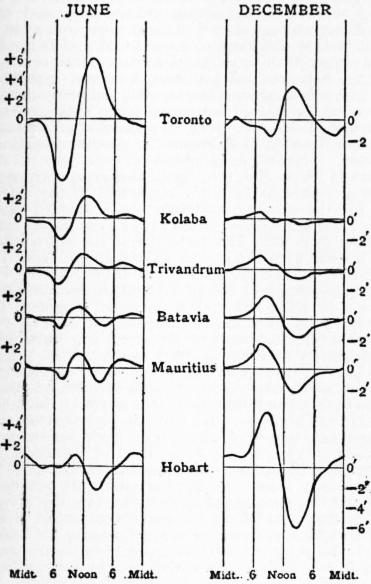
Fig. 6.

With diminishing latitude, there is a gradual transition from the temperate to the tropical type of horizontal force diurnal variation, and at stations whose latitude is under 45° there is a very appreciable variation in type with the season. The mean diurnal variation for the year at Tiflis in Table IX. really represents a struggle between the two types, in which on the whole the temperate type prevails. If we take the diurnal variations at Tiflis for midsummer and midwinter, we find the former essentially of the temperate, the latter essentially of the tropical type. A similar conflict may be seen in the mean diurnal inequality for the year at the Cape of Good Hope, but there the tropical type on the whole predominates, and it prevails more at midwinter than at midsummer. Toronto and Hobart, though similar in latitude to Tiflis, show a closer approach to the temperate type. Still at both stations the hours during which the force is below its mean value tend to extend back towards midnight, especially at midsummer. The amplitude of the horizontal force range appears less at intermediate stations, such as Tiflis, than at stations in either higher or lower latitudes. There is a very great difference in this respect between the north and the south of India.

§ 16. In the case of the vertical force in higher temperate latitudes—at Pavlovsk for instance—the diurnal inequalities from “all” and from “quiet” days differ somewhat widely in amplitude and slightly even in type. In mean latitudes, e.g. at Tiflis, there is often a well marked double period in the mean diurnal inequality for the whole year; but even at Tiflis this is hardly, if at all, apparent in the winter months. In the summer months the double period is distinctly seen at Kew and Greenwich, though the evening maximum is always pre-eminent. Speaking generally, the time of the minimum, or principal minimum, varies much less with the season than that of the maximum. At Kew, for instance, on quiet days the minimum falls between 11 a.m. and noon in almost all the months of the year, but the time of the maximum varies from about 4 p.m. in December to 7 p.m. in June. At Kolaba the time of the minimum is nearly independent of the season; but the changes from positive to negative in the forenoon and from negative to positive in the afternoon are some hours later in winter than in summer. At Batavia the diurnal inequality varies very little in type with the season, and there is little evidence of more than one maximum and minimum in the day. At Batavia, as at Kolaba, negative values occur near noon; but it must be remembered that while at Kolaba and more northern stations vertical force urges the north pole of a magnet downwards, the reverse is true of Batavia, as the dip is southerly. At St Helena vertical force is below its mean value in the forenoon, but the change from − to + occurs at noon, or but little later, both in winter and summer. At the Cape of Good Hope the phenomena at midsummer are similar to those at Kolaba, the force being below its mean value from about 9 a.m. to 3 p.m. and above it throughout the rest of the day; but at midwinter there is a conspicuous double period, the force being below its mean from 1 a.m. to 7 a.m. as well as from 11 a.m. to 3 p.m., and thus resembling the all-day annual results at Greenwich. At Hobart vertical force is below its mean value from 1 a.m. to 9 a.m. at midsummer, and from 4 a.m. to noon at midwinter; while the force is above its mean persistently throughout the afternoon both in summer and winter, there is at midwinter a well marked secondary minimum about 6 p.m., almost the same hour as that at which the maximum for the day is observed in summer.