VOLUME XVII SLICE VIII Matter to Mecklenburg (continued 9)

dt dt dt

(1)

The momentum of a particle is the vector obtained by multiplying the velocity by the mass m. The impulse of a force in any infinitely small interval of time δt is the product of the force into δt; it is to be regarded as a vector. The total impulse in any finite interval of time is the integral of the impulses corresponding to the infinitesimal elements δt into which the interval may be subdivided; the summation of which the integral is the limit is of course to be understood in the vectorial sense.

Newton’s Second Law asserts that change of momentum is equal to the impulse; this is a statement as to equality of vectors and so implies identity of direction as well as of magnitude. If X, Y, Z are the components of force, then considering the changes in an infinitely short time δt we have, by projection on the co-ordinate axes, δ(mu) = Xδt, and so on, or

m du = X, m dv = Y, m dw = Z.

dt dt dt

(2)

For example, the path of a particle projected anyhow under gravity will obviously be confined to the vertical plane through the initial direction of motion. Taking this as the plane xy, with the axis of x drawn horizontally, and that of y vertically upwards, we have X = 0, Y = −mg; so that

d2x = 0, d2y = −g.

dt2 dt2

(3)

The solution is

x = At + B, y = −1⁄2gt2 + Ct + D.

(4)

If the initial values of x, y, ẋ, ẏ are given, we have four conditions to determine the four arbitrary constants A, B, C, D. Thus if the particle start at time t = 0 from the origin, with the component velocities u0, v0, we have

x = u0t, y = v0t − 1⁄2gt2.

(5)

Eliminating t we have the equation of the path, viz.

y = v0 x − gx2 .

u0 2u2

(6)

This is a parabola with vertical axis, of latus-rectum 2u02/g. The range on a horizontal plane through O is got by putting y = 0, viz. it is 2u0v0/g. we denote the resultant velocity at any instant by ṡ we have

ṡ2 = ẋ2 + ẏ2 = ṡ02 − 2gy.

(7)

Another important example is that of a particle subject to an acceleration which is directed always towards a fixed point O and is proportional to the distance from O. The motion will evidently be in one plane, which we take as the plane z = 0. If μ be the acceleration at unit distance, the component accelerations parallel to axes of x and y through O as origin will be −μx, −μy, whence

d2x = −μx, d2y = − μy.

dt2 dt2

(8)

The solution is

x = A cos nt + B sin nt, y = C cos nt + D sin nt,

(9)

where n = √μ. If P be the initial position of the particle, we may conveniently take OP as axis of x, and draw Oy parallel to the direction of motion at P. If OP = a, and ṡ0 be the velocity at P, we have, initially, x = a, y = 0, ẋ = 0, ẏ = ṡ0 whence

x = a cos nt, y = b sin nt,

(10)

if b = ṡ0/n. The path is therefore an ellipse of which a, b are conjugate semi-diameters, and is described in the period 2π/√μ; moreover, the velocity at any point P is equal to √μ·OD, where OD is the semi-diameter conjugate to OP. This type of motion is called elliptic harmonic. If the co-ordinate axes are the principal axes of the ellipse, the angle nt in (10) is identical with the “excentric angle.” The motion of the bob of a “spherical pendulum,” i.e. a simple pendulum whose oscillations are not confined to one vertical plane, is of this character, provided the extreme inclination of the string to the vertical be small. The acceleration is towards the vertical through the point of suspension, and is equal to gr/l, approximately, if r denote distance from this vertical. Hence the path is approximately an ellipse, and the period is 2π √(l/g).

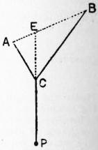
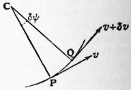
Fig. 65. Fig. 66.

The above problem is identical with that of the oscillation of a particle in a smooth spherical bowl, in the neighbourhood of the lowest point. If the bowl has any other shape, the axes Ox, Oy may be taken tangential to the lines of curvature at the lowest point O; the equations of small motion then are

d2x = −g x , d2y = −g y ,

dt2 ρ1 dt2 ρ2

(11)

where ρ1, ρ2, are the principal radii of curvature at O. The motion is therefore the resultant of two simple vibrations in perpendicular directions, of periods 2π √(ρ1/g), 2π √(ρ2/g). The circumstances are realized in “Blackburn’s pendulum,” which consists of a weight P hanging from a point C of a string ACB whose ends A, B are fixed. If E be the point in which the line of the string meets AB, we have ρ1 = CP, ρ2 = EP. Many contrivances for actually drawing the resulting curves have been devised.

It is sometimes convenient to resolve the accelerations in directions having a more intrinsic relation to the path. Thus, in a plane path, let P, Q be two consecutive positions, corresponding to the times t, t + δt; and let the normals at P, Q meet in C, making an angle δψ. Let v (= ṡ) be the velocity at P, v + δv that at Q. In the time δt the velocity parallel to the tangent at P changes from v to v + δv, ultimately, and the tangential acceleration at P is therefore dv/dt or s̈. Again, the velocity parallel to the normal at P changes from 0 to vδψ, ultimately, so that the normal acceleration is v dψ/dt. Since

dv = dv ds = v dv , v dψ = v dψ ds = v2 ,

dt ds dt ds dt ds dt ρ

(12)

where ρ is the radius of curvature of the path at P, the tangential and normal accelerations are also expressed by v dv/ds and v2/ρ, respectively. Take, for example, the case of a particle moving on a smooth curve in a vertical plane, under the action of gravity and the pressure R of the curve. If the axes of x and y be drawn horizontal and vertical (upwards), and if ψ be the inclination of the tangent to the horizontal, we have

mv dv = − mg sin ψ = − mg dy , mv2 = − mg cos ψ + R.

ds ds ρ

(13)

The former equation gives

v2 = C − 2gy,

(14)

and the latter then determines R.

In the case of the pendulum the tension of the string takes the place of the pressure of the curve. If l be the length of the string, ψ its inclination to the downward vertical, we have δs = lδψ, so that v = ldψ/dt. The tangential resolution then gives

l d2ψ = − g sin ψ.

dt2

(15)

If we multiply by 2dψ/dt and integrate, we obtain

( dψ )2 = 2g cos ψ + const.,

dt l

(16)

which is seen to be equivalent to (14). If the pendulum oscillate between the limits ψ = ±α, we have

( δψ )2 = 2g (cos ψ − cos α) = 4g (sin2 1⁄2α − sin2 1⁄2ψ);

dt l l

(17)

and, putting sin 1⁄2ψ = sin 1⁄2α. sin φ, we find for the period (τ) of a complete oscillation

τ = 4 ∫1⁄2π0 dt dφ = 4√ l · ∫1⁄2π0 dφ

dφ g √(1 − sin2 1⁄2α · sin2 φ)

= 4√ l · F1 (sin 1⁄2α),

g

(18)

in the notation of elliptic integrals. The function F1 (sin β) was tabulated by A. M. Legendre for values of β ranging from 0° to 90°. The following table gives the period, for various amplitudes α, in terms of that of oscillation in an infinitely small arc [viz. 2π√(l/g)] as unit.

α/π τ α/π τ

.1 1.0062 .6 1.2817

.2 1.0253 .7 1.4283

.3 1.0585 .8 1.6551

.4 1.1087 .9 2.0724

.5 1.1804 1.0 ∞

The value of τ can also be obtained as an infinite series, by expanding the integrand in (18) by the binomial theorem, and integrating term by term. Thus

τ = 2π √ l · { 1 + 12 sin2 1⁄2α + 12 · 32 sin4 1⁄2α + ... }.

g 22 22 · 42

(19)

If α be small, an approximation (usually sufficient) is

τ = 2π √(l/g) · (1 + 1⁄16α2).

In the extreme case of α = π, the equation (17) is immediately integrable; thus the time from the lowest position is

t = √(l/g) · log tan (1⁄4π + 1⁄4ψ).

(20)

This becomes infinite for ψ = π, showing that the pendulum only tends asymptotically to the highest position.

The variation of period with amplitude was at one time a hindrance to the accurate performance of pendulum clocks, since the errors produced are cumulative. It was therefore sought to replace the circular pendulum by some other contrivance free from this defect. The equation of motion of a particle in any smooth path is

d2s = −g sin ψ,

dt2

(21)

where ψ is the inclination of the tangent to the horizontal. If sin ψ were accurately and not merely approximately proportional to the arc s, say

s = k sin ψ,

(22)

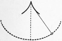
Fig. 67.

the equation (21) would assume the same form as § 12 (5). The motion along the arc would then be accurately simple-harmonic, and the period 2π √(k/g) would be the same for all amplitudes. Now equation (22) is the intrinsic equation of a cycloid; viz. the curve is that traced by a point on the circumference of a circle of radius 1⁄4k which rolls on the under side of a horizontal straight line. Since the evolute of a cycloid is an equal cycloid the object is attained by means of two metal cheeks, having the form of the evolute near the cusp, on which the string wraps itself alternately as the pendulum swings. The device has long been abandoned, the difficulty being met in other ways, but the problem, originally investigated by C. Huygens, is important in the history of mathematics.

The component accelerations of a point describing a tortuous curve, in the directions of the tangent, the principal normal, and the binormal, respectively, are found as follows. If OV>, OV′> be vectors representing the velocities at two consecutive points P, P′ of the path, the plane VOV′ is ultimately parallel to the osculating plane of the path at P; the resultant acceleration is therefore in the osculating plane. Also, the projections of VV′> on OV and on a perpendicular to OV in the plane VOV′ are δv and vδε, where δε is the angle between the directions of the tangents at P, P′. Since δε = δs/ρ, where δs = PP′ = vδt and ρ is the radius of principal curvature at P, the component accelerations along the tangent and principal normal are dv/dt and vdε/dt, respectively, or vdv/ds and v2/ρ. For example, if a particle moves on a smooth surface, under no forces except the reaction of the surface, v is constant, and the principal normal to the path will coincide with the normal to the surface. Hence the path is a “geodesic” on the surface.

If we resolve along the tangent to the path (whether plane or tortuous), the equation of motion of a particle may be written

mv dv = T,

ds

(23)

where T is the tangential component of the force. Integrating with respect to s we find

1⁄2mv12 − 1⁄2mv02 = ∫s1s0 T ds;

(24)

i.e. the increase of kinetic energy between any two positions is equal to the work done by the forces. The result follows also from the Cartesian equations (2); viz. we have

m (ẋẍ + ẏÿ + żz̈) = Xẋ + Yẏ + Zż,

(25)

whence, on integration with respect to t,

1⁄2m (ẋ2 + ẏ2 + ż2) = ∫ (Xẋ + Yẏ + Zż) dt + const.

= ∫ (X dx + Y dy + Z dz) + const.

(26)

If the axes be rectangular, this has the same interpretation as (24).

Suppose now that we have a constant field of force; i.e. the force acting on the particle is always the same at the same place. The work which must be done by forces extraneous to the field in order to bring the particle from rest in some standard position A to rest in any other position P will not necessarily be the same for all paths between A and P. If it is different for different paths, then by bringing the particle from A to P by one path, and back again from P to A by another, we might secure a gain of work, and the process could be repeated indefinitely. If the work required is the same for all paths between A and P, and therefore zero for a closed circuit, the field is said to be conservative. In this case the work required to bring the particle from rest at A to rest at P is called the potential energy of the particle in the position P; we denote it by V. If PP′ be a linear element δs drawn in any direction from P, and S be the force due to the field, resolved in the direction PP′, we have δV = −Sδs or

S = − ∂V .

∂s

(27)

In particular, by taking PP′ parallel to each of the (rectangular) co-ordinate axes in succession, we find

X = − ∂V , Y = − ∂V , Z = − ∂V .

∂x ∂y ∂z

(28)

The equation (24) or (26) now gives

1⁄2mv12 + V1 = 1⁄2mv02 + V0;

(29)

i.e. the sum of the kinetic and potential energies is constant when no work is done by extraneous forces. For example, if the field be that due to gravity we have V = ƒmg dy = mgy + const., if the axis of y be drawn vertically upwards; hence

1⁄2mv2 + mgy = const.

(30)

This applies to motion on a smooth curve, as well as to the free motion of a projectile; cf. (7), (14). Again, in the case of a force Kr towards O, where r denotes distance from O we have V = ∫ Kr dr = 1⁄2Kr2 + const., whence

1⁄2mv2 + 1⁄2Kr2 = const.

(31)

It has been seen that the orbit is in this case an ellipse; also that if we put μ = K/m the velocity at any point P is v = √μ. OD, where OD is the semi-diameter conjugate to OP. Hence (31) is consistent with the known property of the ellipse that OP2 + OD2 is constant.

The forms assumed by the dynamical equations when the axes of reference are themselves in motion will be considered in § 21. At present we take only the case where the rectangular axes Ox, Oy rotate in their own plane, with angular velocity ω about Oz, which is fixed. In the interval δt the projections of the line joining the origin to any point (x, y, z) on the directions of the co-ordinate axes at time t are changed from x, y, z to (x + δx) cos ω δt − (y + δy) sin ωδt, (x + δx) sin ω δt + (y + δy) cos ω δt, z respectively. Hence the component velocities parallel to the instantaneous positions of the co-ordinate axes at time t are

u = ẋ − ωy, v = ẏ + ωz, ω = ż.

(32)

In the same way we find that the component accelerations are

u̇ − ωv, v̇ + ωu, ω̇

(33)

Hence if ω be constant the equations of motion take the forms

m (ẍ − 2ωẏ − ω2ẋ) = X, m (ÿ + 2ωẋ − ω2y) = Y, mz̈ = Z.

(34)

These become identical with the equations of motion relative to fixed axes provided we introduce a fictitious force mω2r acting outwards from the axis of z, where r = √(x2 + y2), and a second fictitious force 2mωv at right angles to the path, where v is the component of the relative velocity parallel to the plane xy. The former force is called by French writers the force centrifuge ordinaire, and the latter the force centrifuge composée, or force de Coriolis. As an application of (34) we may take the case of a symmetrical Blackburn’s pendulum hanging from a horizontal bar which is made to rotate about a vertical axis half-way between the points of attachment of the upper string. The equations of small motion are then of the type

ẍ − 2ωẏ − ω2x = −p2x, ÿ + 2ωẋ − ω2y = −q2y.

(35)

This is satisfied by

ẍ = A cos (σt + ε), y = B sin (σt + ε),

(36)

provided

(σ2 + ω2 − p2) A + 2σωB = 0,

2σωA + (σ2 + ω2 − q2) B = 0.

(37)

Eliminating the ratio A : B we have

(σ2 + ω2 − p2) (σ2 + ω2 − q2) − 4σ2ω2 = 0.

(38)

It is easily proved that the roots of this quadratic in σ2 are always real, and that they are moreover both positive unless ω2 lies between p2 and q2. The ratio B/A is determined in each case by either of the equations (37); hence each root of the quadratic gives a solution of the type (36), with two arbitrary constants A, ε. Since the equations (35) are linear, these two solutions are to be superposed. If the quadratic (38) has a negative root, the trigonometrical functions in (36) are to be replaced by real exponentials, and the position x = 0, y = 0 is unstable. This occurs only when the period (2π/ω) of revolution of the arm lies between the two periods (2π/p, 2π/q) of oscillation when the arm is fixed.

§ 14. Central Forces. Hodograph.—The motion of a particle subject to a force which passes always through a fixed point O is necessarily in a plane orbit. For its investigation we require two equations; these may be obtained in a variety of forms.

Since the impulse of the force in any element of time δt has zero moment about O, the same will be true of the additional momentum generated. Hence the moment of the momentum (considered as a localized vector) about O will be constant. In symbols, if v be the velocity and p the perpendicular from O to the tangent to the path,

pv = h,

(1)

where h is a constant. If δs be an element of the path, pδs is twice the area enclosed by δs and the radii drawn to its extremities from O. Hence if δA be this area, we have δA = 1⁄2 pδs = 1⁄2 hδt, or

dA = 1⁄2h

dt

(2)

Hence equal areas are swept over by the radius vector in equal times.

If P be the acceleration towards O, we have

v dv = −P dr

ds ds

(3)

since dr/ds is the cosine of the angle between the directions of r and δs. We will suppose that P is a function of r only; then integrating (3) we find

1⁄2v2 = − ∫ P dr + const.,

(4)

which is recognized as the equation of energy. Combining this with (1) we have

h2 = C − 2 ∫ P dr,

p2

(5)

which completely determines the path except as to its orientation with respect to O.

If the law of attraction be that of the inverse square of the distance, we have P = μ/r2, and

h2 = C + 2μ .

p2 τ

(6)

Now in a conic whose focus is at O we have

l = 2 ± 1 ,

p2 r a

(7)

where l is half the latus-rectum, a is half the major axis, and the upper or lower sign is to be taken according as the conic is an ellipse or hyperbola. In the intermediate case of the parabola we have a = ∞ and the last term disappears. The equations (6) and (7) are identified by putting

l = h2/μ, a = ± μ/C.

(8)

Since

v2 = h2 = μ ( 2 ± 1 ),

p2 r a

(9)

it appears that the orbit is an ellipse, parabola or hyperbola, according as v2 is less than, equal to, or greater than 2μ/r. Now it appears from (6) that 2μ/r is the square of the velocity which would be acquired by a particle falling from rest at infinity to the distance r. Hence the character of the orbit depends on whether the velocity at any point is less than, equal to, or greater than the velocity from infinity, as it is called. In an elliptic orbit the area πab is swept over in the time

r = πab = 2πa3/2 ,

1⁄2h √μ

(10)

since h = μ1/2l1/2 = μ1/2ba−1/2 by (8).

The converse problem, to determine the law of force under which a given orbit can be described about a given pole, is solved by differentiating (5) with respect to r; thus

P = h2 dp .

p3 dr

(11)

In the case of an ellipse described about the centre as pole we have

a2b2 = a2 + b2 − r2;

p2

(12)

hence P = μr, if μ = h2/a2b2. This merely shows that a particular ellipse may be described under the law of the direct distance provided the circumstances of projection be suitably adjusted. But since an ellipse can always be constructed with a given centre so as to touch a given line at a given point, and to have a given value of ab (= h/√μ) we infer that the orbit will be elliptic whatever the initial circumstances. Also the period is 2πab/h = 2π/√μ, as previously found.

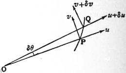
Fig. 68.

Again, in the equiangular spiral we have p = r sinα, and therefore P = μ/r3, if μ = h2/sin2 α. But since an equiangular spiral having a given pole is completely determined by a given point and a given tangent, this type of orbit is not a general one for the law of the inverse cube. In order that the spiral may be described it is necessary that the velocity of projection should be adjusted to make h = √μ·sinα. Similarly, in the case of a circle with the pole on the circumference we have p2 = r2/2a, P = μ/r5, if μ = 8h2a2; but this orbit is not a general one for the law of the inverse fifth power.

In astronomical and other investigations relating to central forces it is often convenient to use polar co-ordinates with the centre of force as pole. Let P, Q be the positions of a moving point at times t, t + δt, and write OP = r, OQ = r + δr, ∠POQ = δθ, O being any fixed origin. If u, v be the component velocities at P along and perpendicular to OP (in the direction of θ increasing), we have

u = lim. δr = dr , v = lim. r δθ = r dθ .

δt dt δt dt

(13)

Again, the velocities parallel and perpendicular to OP change in the time δt from u, v to u − v δθ, v + u δθ, ultimately. The component accelerations at P in these directions are therefore

du − v dθ = d2r − r ( dθ )2,

dt dt dt2 dt

dv + u dθ = 1 d ( r2 dθ ),

dt dt r dt dt

(14)

respectively.

In the case of a central force, with O as pole, the transverse acceleration vanishes, so that

r2 dθ / dt = h,

(15)

where h is constant; this shows (again) that the radius vector sweeps over equal areas in equal times. The radial resolution gives

d2r − r ( dθ )2 = −P,

dt2 dt

(16)

where P, as before, denotes the acceleration towards O. If in this we put r = 1/u, and eliminate t by means of (15), we obtain the general differential equation of central orbits, viz.

d2u + u = P .

dθ2 h2u2

(17)

If, for example, the law be that of the inverse square, we have P = μu2, and the solution is of the form

u = μ {1 + e cos (θ − α)},

h2

(18)

where e, α are arbitrary constants. This is recognized as the polar equation of a conic referred to the focus, the half latus-rectum being h2/μ.

The law of the inverse cube P = μu3 is interesting by way of contrast. The orbits may be divided into two classes according as h2 ≷ μ, i.e. according as the transverse velocity (hu) is greater or less than the velocity √μ·u appropriate to a circular orbit at the same distance. In the former case the equation (17) takes the form

d2u + m2u = 0,

dθ2

(19)

the solution of which is

au = sin m (θ − α).

(20)

The orbit has therefore two asymptotes, inclined at an angle π/m. In the latter case the differential equation is of the form

d2u = m2u,

dθ2

(21)

so that

u = Aemθ + Be−mθ

(22)

If A, B have the same sign, this is equivalent to

au = cosh mθ,

(23)

if the origin of θ be suitably adjusted; hence r has a maximum value α, and the particle ultimately approaches the pole asymptotically by an infinite number of convolutions. If A, B have opposite signs the form is

au = sinh mθ,

(24)

this has an asymptote parallel to θ = 0, but the path near the origin has the same general form as in the case of (23). If A or B vanish we have an equiangular spiral, and the velocity at infinity is zero. In the critical case of h2 = μ, we have d2u/dθ2 = 0, and

u = Aθ + B;

(25)

the orbit is therefore a “reciprocal spiral,” except in the special case of A = 0, when it is a circle. It will be seen that unless the conditions be exactly adjusted for a circular orbit the particle will either recede to infinity or approach the pole asymptotically. This problem was investigated by R. Cotes (1682-1716), and the various curves obtained arc known as Coles’s spirals.

A point on a central orbit where the radial velocity (dr/dt) vanishes is called an apse, and the corresponding radius is called an apse-line. If the force is always the same at the same distance any apse-line will divide the orbit symmetrically, as is seen by imagining the velocity at the apse to be reversed. It follows that the angle between successive apse-lines is constant; it is called the apsidal angle of the orbit.

If in a central orbit the velocity is equal to the velocity from infinity, we have, from (5),

h2 = 2 ∫∞r P dr;

p2

(26)

this determines the form of the critical orbit, as it is called. If P = μ/rn, its polar equation is

rm cos mθ = am,

(27)

where m = 1⁄2(3 − n), except in the case n = 3, when the orbit is an equiangular spiral. The case n = 2 gives the parabola as before.

If we eliminate dθ/dt between (15) and (16) we obtain

d2r − h2 = −P = −ƒ(r),

dt2 r3

say. We may apply this to the investigation of the stability of a circular orbit. Assuming that r = a + x, where x is small, we have, approximately,

d2x − h2 ( 1 − 3x ) = −ƒ(a) − xƒ′(a).

dt2 a3 a

Hence if h and a be connected by the relation h2 = a3ƒ(a) proper to a circular orbit, we have

d2x + { ƒ′(a) + 3 ƒ(a) } x = 0

dt2 a

(28)

If the coefficient of x be positive the variations of x are simple-harmonic, and x can remain permanently small; the circular orbit is then said to be stable. The condition for this may be written

d { a3ƒ(a) } > 0,

da

(29)

i.e. the intensity of the force in the region for which r = a, nearly, must diminish with increasing distance less rapidly than according to the law of the inverse cube. Again, the half-period of x is π / √{ƒ′(a) + 3−1ƒ(a)}, and since the angular velocity in the orbit is h/a2, approximately, the apsidal angle is, ultimately,

π √{ ƒ(a) },

aƒ′(a) + 3ƒ(a)

(30)

or, in the case of ƒ(a) = μ/rn, π/√(3 − n). This is in agreement with the known results for n = 2, n = −1.

We have seen that under the law of the inverse square all finite orbits are elliptical. The question presents itself whether there then is any other law of force, giving a finite velocity from infinity, under which all finite orbits are necessarily closed curves. If this is the case, the apsidal angle must evidently be commensurable with π, and since it cannot vary discontinuously the apsidal angle in a nearly circular orbit must be constant. Equating the expression (30) to π/m, we find that ƒ(a) = C/an, where n = 3 − m2. The force must therefore vary as a power of the distance, and n must be less than 3. Moreover, the case n = 2 is the only one in which the critical orbit (27) can be regarded as the limiting form of a closed curve. Hence the only law of force which satisfies the conditions is that of the inverse square.

At the beginning of § 13 the velocity of a moving point P was represented by a vector OV> drawn from a fixed origin O. The locus of the point V is called the hodograph (q.v.); and it appears that the velocity of the point V along the hodograph represents in magnitude and in direction the acceleration in the original orbit. Thus in the case of a plane orbit, if v be the velocity of P, ψ the inclination of the direction of motion to some fixed direction, the polar co-ordinates of V may be taken to be v, ψ; hence the velocities of V along and perpendicular to OV will be dv/dt and v dψ/dt. These expressions therefore give the tangential and normal accelerations of P; cf. § 13 (12).

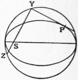
Fig. 69.

In the motion of a projectile under gravity the hodograph is a vertical line described with constant velocity. In elliptic harmonic motion the velocity of P is parallel and proportional to the semi-diameter CD which is conjugate to the radius CP; the hodograph is therefore an ellipse similar to the actual orbit. In the case of a central orbit described under the law of the inverse square we have v = h/SY = h. SZ/b2, where S is the centre of force, SY is the perpendicular to the tangent at P, and Z is the point where YS meets the auxiliary circle again. Hence the hodograph is similar and similarly situated to the locus of Z (the auxiliary circle) turned about S through a right angle. This applies to an elliptic or hyperbolic orbit; the case of the parabolic orbit may be examined separately or treated as a limiting case. The annexed fig. 70 exhibits the various cases, with the hodograph in its proper orientation. The pole O of the hodograph is inside on or outside the circle, according as the orbit is an ellipse, parabola or hyperbola. In any case of a central orbit the hodograph (when turned through a right angle) is similar and similarly situated to the “reciprocal polar” of the orbit with respect to the centre of force. Thus for a circular orbit with the centre of force at an excentric point, the hodograph is a conic with the pole as focus. In the case of a particle oscillating under gravity on a smooth cycloid from rest at the cusp the hodograph is a circle through the pole, described with constant velocity.

§ 15. Kinetics of a System of Discrete Particles.—The momenta of the several particles constitute a system of localized vectors which, for purposes of resolving and taking moments, may be reduced like a system of forces in statics (§ 8). Thus taking any point O as base, we have first a linear momentum whose components referred to rectangular axes through O are

Σ(mẋ), Σ(mẏ), Σ(mż);

(1)

its representative vector is the same whatever point O be chosen. Secondly, we have an angular momentum whose components are

Σ {m (yż − zẏ) }, Σ {m (zẋ − xż) }, Σ {m (xẏ − yẋ) },

(2)

these being the sums of the moments of the momenta of the several particles about the respective axes. This is subject to the same relations as a couple in statics; it may be represented by a vector which will, however, in general vary with the position of O.

The linear momentum is the same as if the whole mass were concentrated at the centre of mass G, and endowed with the velocity of this point. This follows at once from equation (8) of § 11, if we imagine the two configurations of the system there referred to to be those corresponding to the instants t, t + δt. Thus

Σ ( m· PP> ) = Σ(m)· GG′> .

δt δt

(3)

Analytically we have

Σ(mẋ) = d Σ(mx) = Σ(m)· dx ,

dt dt

(4)

with two similar formulae.

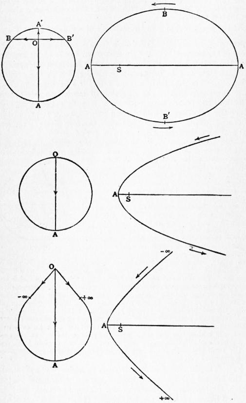
Fig. 70.

Again, if the instantaneous position of G be taken as base, the angular momentum of the absolute motion is the same as the angular momentum of the motion relative to G. For the velocity of a particle m at P may be replaced by two components one of which (v) is identical in magnitude and direction with the velocity of G, whilst the other (v) is the velocity relative to G. The aggregate of the components mv of momentum is equivalent to a single localized vector Σ(m)·v in a line through G, and has therefore zero moment about any axis through G; hence in taking moments about such an axis we need only regard the velocities relative to G. In symbols, we have

Σ { m(yż − zẏ) } = Σ(m)· ( y dz − z dy ) + Σ { m (ηζ − ζ̇η̇) }.

dt dt

(5)

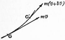
Fig. 71.

since Σ(mξ) = 0, Σ(mξ̇) = 0, and so on, the notation being as in § 11. This expresses that the moment of momentum about any fixed axis (e.g. Ox) is equal to the moment of momentum of the motion relative to G about a parallel axis through G, together with the moment of momentum of the whole mass supposed concentrated at G and moving with this point. If in (5) we make O coincide with the instantaneous position of G, we have x, z, z = 0, and the theorem follows.

Finally, the rates of change of the components of the angular momentum of the motion relative to G referred to G as a moving base, are equal to the rates of change of the corresponding components of angular momentum relative to a fixed base coincident with the instantaneous position of G. For let G′ be a consecutive position of G. At the instant t + δt the momenta of the system are equivalent to a linear momentum represented by a localized vector Σ(m)·(v + δv) in a line through G′ tangential to the path of G′, together with a certain angular momentum. Now the moment of this localized vector with respect to any axis through G is zero, to the first order of δt, since the perpendicular distance of G from the tangent line at G′ is of the order (δt)2. Analytically we have from (5),

d Σ { m (yż − zẏ) } = Σ(m)· ( y dz2 − z d2y ) + d Σ { m(ηζ − ζη̇) }

dt dt2 dt2 dt

(6)

If we put x, y, z = 0, the theorem is proved as regards axes parallel to Ox.

Next consider the kinetic energy of the system. If from a fixed point O we draw vectors OV1>, OV2> to represent the velocities of the several particles m1, m2 ..., and if we construct the vector

OK> = Σ ( m·OV> )

Σ(m)

(7)

this will represent the velocity of the mass-centre, by (3). We find, exactly as in the proof of Lagrange’s First Theorem (§ 11), that

1⁄2Σ (m·OV2) = 1⁄2Σ (m)·OK2 + 1⁄2Σ (m·KV2);

(8)

i.e. the total kinetic energy is equal to the kinetic energy of the whole mass supposed concentrated at G and moving with this point, together with the kinetic energy of the motion relative to G. The latter may be called the internal kinetic energy of the system. Analytically we have

1⁄2Σ { m (ẋ2 + ẏ2 + ż2) } = 1⁄2Σ(m)· { ( dx )2 + ( dy )2 + ( dz )2 } + 1⁄2Σ{ m(ζ2 + η̇2 + ζ̇2) }.

dt dt dt

(9)

There is also an analogue to Lagrange’s Second Theorem, viz.

1⁄2Σ (m·KV2) = 1⁄2 ΣΣ (mpmq · VpVq2) ,

Σm

(10)

which expresses the internal kinetic energy in terms of the relative velocities of the several pairs of particles. This formula is due to Möbius.

The preceding theorems are purely kinematical. We have now to consider the effect of the forces acting on the particles. These may be divided into two categories; we have first, the extraneous forces exerted on the various particles from without, and, secondly, the mutual or internal forces between the various pairs of particles. It is assumed that these latter are subject to the law of equality of action and reaction. If the equations of motion of each particle be formed separately, each such internal force will appear twice over, with opposite signs for its components, viz. as affecting the motion of each of the two particles between which it acts. The full working out is in general difficult, the comparatively simple problem of “three bodies,” for instance, in gravitational astronomy being still unsolved, but some general theorems can be formulated.

The first of these may be called the Principle of Linear Momentum. If there are no extraneous forces, the resultant linear momentum is constant in every respect. For consider any two particles at P and Q, acting on one another with equal and opposite forces in the line PQ. In the time δt a certain impulse is given to the first particle in the direction (say) from P to Q, whilst an equal and opposite impulse is given to the second in the direction from Q to P. Since these impulses produce equal and opposite momenta in the two particles, the resultant linear momentum of the system is unaltered. If extraneous forces act, it is seen in like manner that the resultant linear momentum of the system is in any given time modified by the geometric addition of the total impulse of the extraneous forces. It follows, by the preceding kinematic theory, that the mass-centre G of the system will move exactly as if the whole mass were concentrated there and were acted on by the extraneous forces applied parallel to their original directions. For example, the mass-centre of a system free from extraneous force will describe a straight line with constant velocity. Again, the mass-centre of a chain of particles connected by strings, projected anyhow under gravity, will describe a parabola.

The second general result is the Principle of Angular Momentum. If there are no extraneous forces, the moment of momentum about any fixed axis is constant. For in time δt the mutual action between two particles at P and Q produces equal and opposite momenta in the line PQ, and these will have equal and opposite moments about the fixed axis. If extraneous forces act, the total angular momentum about any fixed axis is in time δt increased by the total extraneous impulse about that axis. The kinematical relations above explained now lead to the conclusion that in calculating the effect of extraneous forces in an infinitely short time δt we may take moments about an axis passing through the instantaneous position of G exactly as if G were fixed; moreover, the result will be the same whether in this process we employ the true velocities of the particles or merely their velocities relative to G. If there are no extraneous forces, or if the extraneous forces have zero moment about any axis through G, the vector which represents the resultant angular momentum relative to G is constant in every respect. A plane through G perpendicular to this vector has a fixed direction in space, and is called the invariable plane; it may sometimes be conveniently used as a plane of reference.

For example, if we have two particles connected by a string, the invariable plane passes through the string, and if ω be the angular velocity in this plane, the angular momentum relative to G is

m1ω1r1·r1 + m2ωr2·r2 = (m1r12 + m2r22) ω,

where r1, r2 are the distances of m1, m2 from their mass-centre G. Hence if the extraneous forces (e.g. gravity) have zero moment about G, ω will be constant. Again, the tension R of the string is given by

R = m1ω2r1 = m1m2 ω2a,

m1 + m2

where a = r1 + r2. Also by (10) the internal kinetic energy is

1⁄2 m1m2 ω2a2

m1 + m2

The increase of the kinetic energy of the system in any interval of time will of course be equal to the total work done by all the forces acting on the particles. In many questions relating to systems of discrete particles the internal force Rpq (which we will reckon positive when attractive) between any two particles mp, mq is a function only of the distance rpq between them. In this case the work done by the internal forces will be represented by

−Σ ∫ Rpg drpq,

when the summation includes every pair of particles, and each integral is to be taken between the proper limits. If we write

V = Σ ∫ Rpq drpq,

(11)

when rpq ranges from its value in some standard configuration A of the system to its value in any other configuration P, it is plain that V represents the work which would have to be done in order to bring the system from rest in the configuration A to rest in the configuration P. Hence V is a definite function of the configuration P; it is called the internal potential energy. If T denote the kinetic energy, we may say then that the sum T + V is in any interval of time increased by an amount equal to the work done by the extraneous forces. In particular, if there are no extraneous forces T + V is constant. Again, if some of the extraneous forces are due to a conservative field of force, the work which they do may be reckoned as a diminution of the potential energy relative to the field as in § 13.

§ 16. Kinetics of a Rigid Body. Fundamental Principles.—When we pass from the consideration of discrete particles to that of continuous distributions of matter, we require some physical postulate over and above what is contained in the Laws of Motion, in their original formulation. This additional postulate may be introduced under various forms. One plan is to assume that any body whatever may be treated as if it were composed of material particles, i.e. mathematical points endowed with inertia coefficients, separated by finite intervals, and acting on one another with forces in the lines joining them subject to the law of equality of action and reaction. In the case of a rigid body we must suppose that those forces adjust themselves so as to preserve the mutual distances of the various particles unaltered. On this basis we can predicate the principles of linear and angular momentum, as in § 15.

An alternative procedure is to adopt the principle first formally enunciated by J. Le R. d’Alembert and since known by his name. If x, y, z be the rectangular co-ordinates of a mass-element m, the expressions mẍ, mÿ, mz̈ must be equal to the components of the total force on m, these forces being partly extraneous and partly forces exerted on m by other mass-elements of the system. Hence (mẍ, mÿ, mz̈) is called the actual or effective force on m. According to d’Alembert’s formulation, the extraneous forces together with the effective forces reversed fulfil the statical conditions of equilibrium. In other words, the whole assemblage of effective forces is statically equivalent to the extraneous forces. This leads, by the principles of § 8, to the equations

Σ(mẍ) = X, Σ(mÿ) = Y, Σ(mz̈) = Z, Σ {m (yz̈ − zÿ) } = L, Σ {m (zẍ − xz̈) } = M, Σ{m (xÿ − yẍ) } = N,

(1)

where (X, Y, Z) and (L, M, N) are the force—and couple—constituents of the system of extraneous forces, referred to O as base, and the summations extend over all the mass-elements of the system. These equations may be written

d Σ(mẋ) = X, d Σ(mẏ) = Y, d Σ(mż) = Z,

dt dt dt

d Σ {m (yż − zẏ) } = L, d Σ {m (zẋ − xż) } = M, d Σ {m (xẏ − yẋ) } = N,

dt dt dt

(2)

and so express that the rate of change of the linear momentum in any fixed direction (e.g. that of Ox) is equal to the total extraneous force in that direction, and that the rate of change of the angular momentum about any fixed axis is equal to the moment of the extraneous forces about that axis. If we integrate with respect to t between fixed limits, we obtain the principles of linear and angular momentum in the form previously given. Hence, whichever form of postulate we adopt, we are led to the principles of linear and angular momentum, which form in fact the basis of all our subsequent work. It is to be noticed that the preceding statements are not intended to be restricted to rigid bodies; they are assumed to hold for all material systems whatever. The peculiar status of rigid bodies is that the principles in question are in most cases sufficient for the complete determination of the motion, the dynamical equations (1 or 2) being equal in number to the degrees of freedom (six) of a rigid solid, whereas in cases where the freedom is greater we have to invoke the aid of other supplementary physical hypotheses (cf. Elasticity; Hydromechanics).

The increase of the kinetic energy of a rigid body in any interval of time is equal to the work done by the extraneous forces acting on the body. This is an immediate consequence of the fundamental postulate, in either of the forms above stated, since the internal forces do on the whole no work. The statement may be extended to a system of rigid bodies, provided the mutual reactions consist of the stresses in inextensible links, or the pressures between smooth surfaces, or the reactions at rolling contacts (§ 9).

§ 17. Two-dimensional Problems.—In the case of rotation about a fixed axis, the principles take a very simple form. The position of the body is specified by a single co-ordinate, viz. the angle θ through which some plane passing through the axis and fixed in the body has turned from a standard position in space. Then dθ/dt, = ω say, is the angular velocity of the body. The angular momentum of a particle m at a distance r from the axis is mωr·r, and the total angular momentum is Σ(mr2)·ω, or Iω, if I denote the moment of inertia (§ 11) about the axis. Hence if N be the moment of the extraneous forces about the axis, we have

d (Iω) = N.

dt

(1)

This may be compared with the equation of rectilinear motion of a particle, viz. d/dt·(Mu) = X; it shows that I measures the inertia of the body as regards rotation, just as M measures its inertia as regards translation. If N = 0, ω is constant.

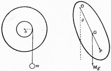
Fig. 72. Fig. 73.

As a first example, suppose we have a flywheel free to rotate about a horizontal axis, and that a weight m hangs by a vertical string from the circumferences of an axle of radius b (fig. 72). Neglecting frictional resistance we have, if R be the tension of the string,

Iω̇ = Rb, mu̇ = mg − R,

whence

bω̇ = mb2 g.

1 + mb2

(2)

This gives the acceleration of m as modified by the inertia of the wheel.

A “compound pendulum” is a body of any form which is free to rotate about a fixed horizontal axis, the only extraneous force (other than the pressures of the axis) being that of gravity. If M be the total mass, k the radius of gyration (§ 11) about the axis, we have

d ( Mk2 dθ ) = −Mgh sin θ,

dt dt

(3)

where θ is the angle which the plane containing the axis and the centre of gravity G makes with the vertical, and h is the distance of G from the axis. This coincides with the equation of motion of a simple pendulum [§ 13 (15)] of length l, provided l = k2/h. The plane of the diagram (fig. 73) is supposed to be a plane through G perpendicular to the axis, which it meets in O. If we produce OG to P, making OP = l, the point P is called the centre of oscillation; the bob of a simple pendulum of length OP suspended from O will keep step with the motion of P, if properly started. If κ be the radius of gyration about a parallel axis through G, we have k2 = κ2 + h2 by § 11 (16), and therefore l = h + κ2/h, whence

GO · GP = κ2.

(4)

This shows that if the body were swung from a parallel axis through P the new centre of oscillation would be at O. For different parallel axes, the period of a small oscillation varies as √l, or √(GO + OP); this is least, subject to the condition (4), when GO = GP = κ. The reciprocal relation between the centres of suspension and oscillation is the basis of Kater’s method of determining g experimentally. A pendulum is constructed with two parallel knife-edges as nearly as possible in the same plane with G, the position of one of them being adjustable. If it could be arranged that the period of a small oscillation should be exactly the same about either edge, the two knife-edges would in general occupy the positions of conjugate centres of suspension and oscillation; and the distances between them would be the length l of the equivalent simple pendulum. For if h1 + κ2/h1 = h2 + κ2/h2, then unless h1 = h2, we must have κ2 = h1h2, l = h1 + h2. Exact equality of the two observed periods (τ1, τ2, say) cannot of course be secured in practice, and a modification is necessary. If we write l1 = h1 + κ2/h1, l2 = h2 + κ2/h2, we find, on elimination of κ,

1⁄2 l1 + l2 + 1⁄2 l1 − l2 = 1,

h1 + h2 h1 − h2

whence

4π2 = 1⁄2 (τ12 + τ22) + 1⁄2 (τ12 − τ22) .

g h1 + h2 h1 − h2

(5)

The distance h1 + h2, which occurs in the first term on the right hand can be measured directly. For the second term we require the values of h1, h2 separately, but if τ1, τ2 are nearly equal whilst h1, h2 are distinctly unequal this term will be relatively small, so that an approximate knowledge of h1, h2 is sufficient.

As a final example we may note the arrangement, often employed in physical measurements, where a body performs small oscillations about a vertical axis through its mass-centre G, under the influence of a couple whose moment varies as the angle of rotation from the equilibrium position. The equation of motion is of the type

I θ̈ = −Kθ,

(6)

and the period is therefore τ = 2π√(I/K). If by the attachment of another body of known moment of inertia I′, the period is altered from τ to τ′, we have τ′ = 2π√{ (I + I′)/K }. We are thus enabled to determine both I and K, viz.

I / I′ = τ2 / (τ′2 − τ2), K = 4π2τ2I / (τ′2 − τ2).

(7)

The couple may be due to the earth’s magnetism, or to the torsion of a suspending wire, or to a “bifilar” suspension. In the latter case, the body hangs by two vertical threads of equal length l in a plane through G. The motion being assumed to be small, the tensions of the two strings may be taken to have their statical values Mgb/(a + b), Mga/(a + b), where a, b are the distances of G from the two threads. When the body is twisted through an angle θ the threads make angles aθ/l, bθ/l with the vertical, and the moment of the tensions about the vertical through G is accordingly −Kθ, where K = M gab/l.

For the determination of the motion it has only been necessary to use one of the dynamical equations. The remaining equations serve to determine the reactions of the rotating body on its bearings. Suppose, for example, that there are no extraneous forces. Take rectangular axes, of which Oz coincides with the axis of rotation. The angular velocity being constant, the effective force on a particle m at a distance r from Oz is mω2r towards this axis, and its components are accordingly −ω2mx, −ω2my, O. Since the reactions on the bearings must be statically equivalent to the whole system of effective forces, they will reduce to a force (X Y Z) at O and a couple (L M N) given by

X = −ω2Σ(mx) = −ω2Σ(m)x, Y = −ω2Σ(my) = −ω2Σ(m)y, Z = 0, L = ω2Σ(myz), M = −ω2Σ(mzx), N = 0,

(8)

where x, y refer to the mass-centre G. The reactions do not therefore reduce to a single force at O unless Σ(myz) = 0, Σ(msx) = 0, i.e. unless the axis of rotation be a principal axis of inertia (§ 11) at O. In order that the force may vanish we must also have x, y = 0, i.e. the mass-centre must lie in the axis of rotation. These considerations are important in the “balancing” of machinery. We note further that if a body be free to turn about a fixed point O, there are three mutually perpendicular lines through this point about which it can rotate steadily, without further constraint. The theory of principal or “permanent” axes was first investigated from this point of view by J. A. Segner (1755). The origin of the name “deviation moment” sometimes applied to a product of inertia is also now apparent.

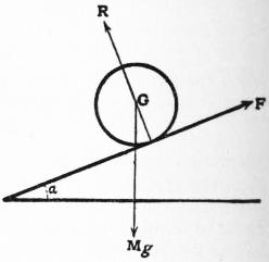
Fig. 74.

Proceeding to the general motion of a rigid body in two dimensions we may take as the three co-ordinates of the body the rectangular Cartesian co-ordinates x, y of the mass-centre G and the angle θ through which the body has turned from some standard position. The components of linear momentum are then Mẋ, Mẏ, and the angular momentum relative to G as base is Iθ̇, where M is the mass and I the moment of inertia about G. If the extraneous forces be reduced to a force (X, Y) at G and a couple N, we have

Mẍ = X, Mÿ = Y, Iθ̈ = N.

(9)

If the extraneous forces have zero moment about G the angular velocity θ̇ is constant. Thus a circular disk projected under gravity in a vertical plane spins with constant angular velocity, whilst its centre describes a parabola.

We may apply the equations (9) to the case of a solid of revolution rolling with its axis horizontal on a plane of inclination α. If the axis of x be taken parallel to the slope of the plane, with x increasing downwards, we have

Mẍ = Mg sin α − F, 0 = Mg cos α − R, Mκ2θ̈ = Fa,

(10)

where κ is the radius of gyration about the axis of symmetry, a is the constant distance of G from the plane, and R, F are the normal and tangential components of the reaction of the plane, as shown in fig. 74. We have also the kinematical relation ẋ = aθ̇. Hence

ẍ = a2 g sin α, R = Mg cos α, F = κ2 Mg sin α.

κ2 + a2 κ2 + a2

(11)

The acceleration of G is therefore less than in the case of frictionless sliding in the ratio a2/(κ2 + a2). For a homogeneous sphere this ratio is 5⁄7, for a uniform circular cylinder or disk 2⁄3, for a circular hoop or a thin cylindrical shell 1⁄2.

The equation of energy for a rigid body has already been stated (in effect) as a corollary from fundamental assumptions. It may also be deduced from the principles of linear and angular momentum as embodied in the equations (9). We have

M (ẋẍ + ẏÿ) + lθ̇θ̈ + Xẋ + Yẏ + Nθ̇,

(12)

whence, integrating with respect to t,

1⁄2M (ẋ2 + ẏ2) + 1⁄2Iθ̇2 = ∫ (X dx + Y dy + N dθ) + const.

(13)

The left-hand side is the kinetic energy of the whole mass, supposed concentrated at G and moving with this point, together with the kinetic energy of the motion relative to G (§ 15); and the right-hand member represents the integral work done by the extraneous forces in the successive infinitesimal displacements into which the motion may be resolved.

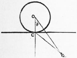
Fig. 75.

The formula (13) may be easily verified in the case of the compound pendulum, or of the solid rolling down an incline. As another example, suppose we have a circular cylinder whose mass-centre is at an excentric point, rolling on a horizontal plane. This includes the case of a compound pendulum in which the knife-edge is replaced by a cylindrical pin. If α be the radius of the cylinder, h the distance of G from its axis (O), κ the radius of gyration about a longitudinal axis through G, and θ the inclination of OG to the vertical, the kinetic energy is 1⁄2Mκ2θ̇2 + 1⁄2M·CG2·thetȧ2, by § 3, since the body is turning about the line of contact (C) as instantaneous axis, and the potential energy is −Mgh cos θ. The equation of energy is therefore

1⁄2M (κ2 + α2 + h2 − 2 ah cos θ) θ̇2 − Mgh cos θ − const.

(14)

Whenever, as in the preceding examples, a body or a system of bodies, is subject to constraints which leave it virtually only one degree of freedom, the equation of energy is sufficient for the complete determination of the motion. If q be any variable co-ordinate defining the position or (in the case of a system of bodies) the configuration, the velocity of each particle at any instant will be proportional to q̇, and the total kinetic energy may be expressed in the form 1⁄2Aq̇2, where A is in general a function of q [cf. equation (14)]. This coefficient A is called the coefficient of inertia, or the reduced inertia of the system, referred to the co-ordinate q.

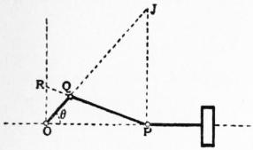
Fig. 76.

Thus in the case of a railway truck travelling with velocity u the kinetic energy is 1⁄2 (M + mκ2/α2)u2, where M is the total mass, α the radius and κ the radius of gyration of each wheel, and m is the sum of the masses of the wheels; the reduced inertia is therefore M + mκ2/α2. Again, take the system composed of the flywheel, connecting rod, and piston of a steam-engine. We have here a limiting case of three-bar motion (§ 3), and the instantaneous centre J of the connecting-rod PQ will have the position shown in the figure. The velocities of P and Q will be in the ratio of JP to JQ, or OR to OQ; the velocity of the piston is therefore yθ̇, where y = OR. Hence if, for simplicity, we neglect the inertia of the connecting-rod, the kinetic energy will be 1⁄2 (I + My2)thetȧ2, where I is the moment of inertia of the flywheel, and M is the mass of the piston. The effect of the mass of the piston is therefore to increase the apparent moment of inertia of the flywheel by the variable amount My2. If, on the other hand, we take OP (= x) as our variable, the kinetic energy is 1⁄2 (M + I/y2)ẋ2. We may also say, therefore, that the effect of the flywheel is to increase the apparent mass of the piston by the amount I/y2; this becomes infinite at the “dead-points” where the crank is in line with the connecting-rod.

If the system be “conservative,” we have

1⁄2Aq2 + V = const.,

(15)

where V is the potential energy. If we differentiate this with respect to t, and divide out by q̇, we obtain

Aq̈ + 1⁄2 dA q̇2 + dV = 0

dq dq

(16)

as the equation of motion of the system with the unknown reactions (if any) eliminated. For equilibrium this must be satisfied by q̇ = O; this requires that dV/dq = 0, i.e. the potential energy must be “stationary.” To examine the effect of a small disturbance from equilibrium we put V = ƒ(q), and write q = q0 + η, where q0 is a root of ƒ′ (q0) = 0 and η is small. Neglecting terms of the second order in η we have dV/dq = ƒ′(q) = ƒ″(q0)·η, and the equation (16) reduces to

Aη̈ + ƒ″ (q0)η = 0,

(17)

where A may be supposed to be constant and to have the value corresponding to q = q0. Hence if ƒ″ (q0) > 0, i.e. if V is a minimum in the configuration of equilibrium, the variation of η is simple-harmonic, and the period is 2π √{A/ƒ″(q0) }. This depends only on the constitution of the system, whereas the amplitude and epoch will vary with the initial circumstances. If ƒ″ (q0) < 0, the solution of (17) will involve real exponentials, and η will in general increase until the neglect of the terms of the second order is no longer justified. The configuration q = q0, is then unstable.

As an example of the method, we may take the problem to which equation (14) relates. If we differentiate, and divide by θ, and retain only the terms of the first order in θ, we obtain

{x2 + (h − α)2} θ̈ + ghθ = 0,

(18)

as the equation of small oscillations about the position θ = 0. The length of the equivalent simple pendulum is {κ2 + (h − α)2}/h.

The equations which express the change of motion (in two dimensions) due to an instantaneous impulse are of the forms

M (u′ − u) = ξ, M (ν′ − ν) = η, I (ω′ − ω) = ν.

(19)

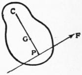
Fig. 77.

Here u′, ν′ are the values of the component velocities of G just before, and u, ν their values just after, the impulse, whilst ω′, ω denote the corresponding angular velocities. Further, ξ, η are the time-integrals of the forces parallel to the co-ordinate axes, and ν is the time-integral of their moment about G. Suppose, for example, that a rigid lamina at rest, but free to move, is struck by an instantaneous impulse F in a given line. Evidently G will begin to move parallel to the line of F; let its initial velocity be u′, and let ω′ be the initial angular velocity. Then Mu′ = F, Iω′ = F·GP, where GP is the perpendicular from G to the line of F. If PG be produced to any point C, the initial velocity of the point C of the lamina will be

u′ − ω′·GC = (F/M) · (I − GC·CP/κ2),

where κ2 is the radius of gyration about G. The initial centre of rotation will therefore be at C, provided GC·GP = κ2. If this condition be satisfied there would be no impulsive reaction at C even if this point were fixed. The point P is therefore called the centre of percussion for the axis at C. It will be noted that the relation between C and P is the same as that which connects the centres of suspension and oscillation in the compound pendulum.

§ 18. Equations of Motion in Three Dimensions.—It was proved in § 7 that a body moving about a fixed point O can be brought from its position at time t to its position at time t + δt by an infinitesimal rotation ε about some axis through O; and the limiting position of this axis, when δt is infinitely small, was called the “instantaneous axis.” The limiting value of the ratio ε/δt is called the angular velocity of the body; we denote it by ω. If ξ, η, ζ are the components of ε about rectangular co-ordinate axes through O, the limiting values of ξ/δt, η/δt, ζ/δt are called the component angular velocities; we denote them by p, q, r. If l, m, n be the direction-cosines of the instantaneous axis we have

p = lω, q = mω, r = nω,

(1)

p2 + q2 + r2 = ω2.

(2)

If we draw a vector OJ to represent the angular velocity, then J traces out a certain curve in the body, called the polhode, and a certain curve in space, called the herpolhode. The cones generated by the instantaneous axis in the body and in space are called the polhode and herpolhode cones, respectively; in the actual motion the former cone rolls on the latter (§ 7).

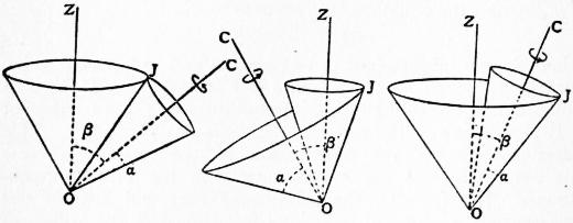
Fig. 78.

The special case where both cones are right circular and ω is constant is important in astronomy and also in mechanism (theory of bevel wheels). The “precession of the equinoxes” is due to the fact that the earth performs a motion of this kind about its centre, and the whole class of such motions has therefore been termed precessional. In fig. 78, which shows the various cases, OZ is the axis of the fixed and OC that of the rolling cone, and J is the point of contact of the polhode and herpolhode, which are of course both circles. If αbe the semi-angle of the rolling cone, β the constant inclination of OC to OZ, and ψ̇ the angular velocity with which the plane ZOC revolves about OZ, then, considering the velocity of a point in OC at unit distance from O, we have

ω sin α = ±ψ̇ sin β,

(3)

where the lower sign belongs to the third case. The earth’s precessional motion is of this latter type, the angles being α = .0087″, β = 23° 28′.

If m be the mass of a particle at P, and PN the perpendicular to the instantaneous axis, the kinetic energy T is given by

2T = Σ {m (ω·PN)2 } = ω2·Σ (m·PN2) = Iω2,

(4)

where I is the moment of inertia about the instantaneous axis. With the same notation for moments and products of inertia as in § 11 (38), we have

I = Al2 + Bm2 + Cn2 − 2Fmn − 2Gnl − 2Hlm,

and therefore by (1),

2T = Ap2 + Bq2 + Cr2 − 2Fqr − 2Grp − 2Hpq.

(5)

Again, if x, y, z be the co-ordinates of P, the component velocities of m are

qz − ry, rx − pz, py − qx,

(6)

by § 7 (5); hence, if λ, μ, ν be now used to denote the component angular momenta about the co-ordinate axes, we have λ = Σ {m (py − qx)y − m(rx − pz) z }, with two similar formulae, or

λ = Ap −Hq − Gr = ∂T ,

∂p

μ = −Hp + Bq − Fr = ∂T ,

∂q

ν = −Gp − Fq + Cr = ∂T .

∂r

(7)

If the co-ordinate axes be taken to coincide with the principal axes of inertia at O, at the instant under consideration, we have the simpler formulae

2T = Ap2 + Bq2 + Cr2,

(8)

λ = Ap, μ = Bq, ν = Cr.

(9)

It is to be carefully noticed that the axis of resultant angular momentum about O does not in general coincide with the instantaneous axis of rotation. The relation between these axes may be expressed by means of the momental ellipsoid at O. The equation of the latter, referred to its principal axes, being as in § 11 (41), the co-ordinates of the point J where it is met by the instantaneous axis are proportional to p, q, r, and the direction-cosines of the normal at J are therefore proportional to Ap, Bq, Cr, or λ, μ, ν. The axis of resultant angular momentum is therefore normal to the tangent plane at J, and does not coincide with OJ unless the latter be a principal axis. Again, if Γ be the resultant angular momentum, so that

λ2 + μ2 + ν2 = Γ2,

(10)

the length of the perpendicular OH on the tangent plane at J is

OH = Ap · p ρ + Bq · q ρ + Cr · r ρ = 2T · ρ ,

Γ ω Γ ω Γ ω Γ ω

(11)

where ρ = OJ. This relation will be of use to us presently (§ 19).

The motion of a rigid body in the most general case may be specified by means of the component velocities u, v, w of any point O of it which is taken as base, and the component angular velocities p, q, r. The component velocities of any point whose co-ordinates relative to O are x, y, z are then

u + qz − ry, v + rx − pz, w + py − qx

(12)

by § 7 (6). It is usually convenient to take as our base-point the mass-centre of the body. In this case the kinetic energy is given by

2T = M0 (u2 + v2 + w2) + Ap2 + Bq2 + Cr2 − 2Fqr − 2Grp − 2Hpg,

(13)

where M0 is the mass, and A, B, C, F, G, H are the moments and products of inertia with respect to the mass-centre; cf. § 15 (9).

The components ξ, η, ζ of linear momentum are

ξ = M0u = ∂T , η = M0v = ∂T , ζ = M0w = ∂T

∂u ∂v ∂w

(14)

whilst those of the relative angular momentum are given by (7). The preceding formulae are sufficient for the treatment of instantaneous impulses. Thus if an impulse (ξ, η, ζ, λ, μ, ν) change the motion from (u, v, w, p, q, r) to (u′, v′, w′, p′, q′, r′) we have

M0 (u′ − u) = ξ, M0 (v′ − v) = η, M0(w′ − w) = ζ,

A (p′ − p) = λ, B (q′ − q) = μ, C (r′ − r) = ν,

(15)

where, for simplicity, the co-ordinate axes are supposed to coincide with the principal axes at the mass-centre. Hence the change of kinetic energy is

T′ − T = ξ · 1⁄2 (u + u′) + η · 1⁄2 (v + v′) + ζ · 1⁄2 (w + w′), + λ · 1⁄2 (p + p′) + μ · 1⁄2 (q + q′) + ν · 1⁄2 (r + r′).

(16)

The factors of ξ, η, ζ, λ, μ, ν on the right-hand side are proportional to the constituents of a possible infinitesimal displacement of the solid, and the whole expression is proportional (on the same scale) to the work done by the given system of impulsive forces in such a displacement. As in § 9 this must be equal to the total work done in such a displacement by the several forces, whatever they are, which make up the impulse. We are thus led to the following statement: the change of kinetic energy due to any system of impulsive forces is equal to the sum of the products of the several forces into the semi-sum of the initial and final velocities of their respective points of application, resolved in the directions of the forces. Thus in the problem of fig. 77 the kinetic energy generated is 1⁄2M (κ2 + Cq2)ω′2, if C be the instantaneous centre; this is seen to be equal to 1⁄2F·ω′·CP, where ω′·CP represents the initial velocity of P.

The equations of continuous motion of a solid are obtained by substituting the values of ξ, η, ζ, λ, μ, ν from (14) and (7) in the general equations

dξ = X, dη = Y, dζ = Z,

dt dt dt

dλ = L, dμ = M, dν = N,

dt dt dt

(17)

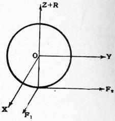
Fig. 79.

where (X, Y, Z, L, M, N) denotes the system of extraneous forces referred (like the momenta) to the mass-centre as base, the co-ordinate axes being of course fixed in direction. The resulting equations are not as a rule easy of application, owing to the fact that the moments and products of inertia A, B, C, F, G, H are not constants but vary in consequence of the changing orientation of the body with respect to the co-ordinate axes.

An exception occurs, however, in the case of a solid which is kinetically symmetrical (§ 11) about the mass-centre, e.g. a uniform sphere. The equations then take the forms

M0u̇ = X, M0v̇ = Y, M0ẇ = Z,

Cṗ = L, Cq̇ = M, Cṙ = N,

(18)

where C is the constant moment of inertia about any axis through the mass-centre. Take, for example, the case of a sphere rolling on a plane; and let the axes Ox, Oy be drawn through the centre parallel to the plane, so that the equation of the latter is z = −a. We will suppose that the extraneous forces consist of a known force (X, Y, Z) at the centre, and of the reactions (F1, F2, R) at the point of contact. Hence

M0u̇ = X + F1, M0v̇ = Y + F2, 0 = Z + R, Cṗ = F2a, Cq̇ = −F1a, Cṙ = 0.

(19)

The last equation shows that the angular velocity about the normal to the plane is constant. Again, since the point of the sphere which is in contact with the plane is instantaneously at rest, we have the geometrical relations

u + qa = 0, v + pa = 0, w = 0,

(20)

by (12). Eliminating p, q, we get

(M0 + Ca−2) u̇ = X, (M0 + Ca−2) v̇ = Y.

(21)

The acceleration of the centre is therefore the same as if the plane were smooth and the mass of the sphere were increased by C/α2. Thus the centre of a sphere rolling under gravity on a plane of inclination a describes a parabola with an acceleration

g sin α/(1 + C/Ma2)

parallel to the lines of greatest slope.

Take next the case of a sphere rolling on a fixed spherical surface. Let a be the radius of the rolling sphere, c that of the spherical surface which is the locus of its centre, and let x, y, z be the co-ordinates of this centre relative to axes through O, the centre of the fixed sphere. If the only extraneous forces are the reactions (P, Q, R) at the point of contact, we have

M0ẍ = P, M0ÿ = Q, M0z̈ = R,

Cṗ = − a (yR − zQ), Cq̇ = − a (zP − xR), Cṙ = − a (xQ − yP),

c c c

(22)

the standard case being that where the rolling sphere is outside the fixed surface. The opposite case is obtained by reversing the sign of a. We have also the geometrical relations

ẋ = (a/c) (qz − ry), ẏ = (a/c) (rx − pz), ż = (a/c) (py − gx),

(23)

If we eliminate P, Q, R from (22), the resulting equations are integrable with respect to t; thus

p = − M0a (yż − zẏ) + α, q = − M0a (zẋ − xż) + β, r = − M0a (xẏ − yẋ) + γ,

Cc Cc Cc

(24)

where α, β, γ are arbitrary constants. Substituting in (23) we find

( 1 + M0a2 ) ẋ = a (βz − γy), ( 1 + M0a2 ) ẏ = a (γx − αz), ( 1 + M0a2 ) ż = a (αy − βx).

C c C c C c

(25)

Hence αẋ + βẏ + γż = 0, or

αx + βy + γz = const.;

(26)

which shows that the centre of the rolling sphere describes a circle. If the axis of z be taken normal to the plane of this circle we have α = 0, β = 0, and

( 1 + M0a2 ) ẋ = −γ a y, ( 1 + M0a2 ) ẏ = γ a x.

C c C c

(27)

The solution of these equations is of the type

x = b cos (στ + ε), y = b sin (σt + ε),

(28)

where b, ε are arbitrary, and

σ = γa/c .

1 + M0a2/C

(29)

The circle is described with the constant angular velocity σ.

When the gravity of the rolling sphere is to be taken into account the preceding method is not in general convenient, unless the whole motion of G is small. As an example of this latter type, suppose that a sphere is placed on the highest point of a fixed sphere and set spinning about the vertical diameter with the angular velocity n; it will appear that under a certain condition the motion of G consequent on a slight disturbance will be oscillatory. If Oz be drawn vertically upwards, then in the beginning of the disturbed motion the quantities x, y, p, q, P, Q will all be small. Hence, omitting terms of the second order, we find

M0ẍ = P, M0ẏ = Q, R = M0g, Cṗ = −(M0ga/c) y + aQ, Cq̇ = (M0ga/c) x − aP, Cṙ = 0.

(30)

The last equation shows that the component r of the angular velocity retains (to the first order) the constant value n. The geometrical relations reduce to

ẋ = aq − (na/c) y, ẏ = −ap + (na/c) x.

(31)

Eliminating p, g, P, Q, we obtain the equations

(C + M0a2) ẍ + (Cna/c) y − (M0ga2/c) x = 0, (C + M0a2) ÿ − (Cna/c) x − (M0ga2/c) y = 0,

(32)

which are both contained in

{ (C + M0a2) d2 − i Cna d − M0ga2 } (x + iy) = 0.

dt2 c dt c

(33)

This has two solutions of the type x + iy = αei(σt + ε), where α, ε are arbitrary, and σ is a root of the quadratic

(C + M0a2) σ2 − (Cna/c) σ + M0ga2/c = 0.

(34)

If

n2 > (4Mgc/C) (1 + M0a2/C),

(35)

both roots are real, and have the same sign as n. The motion of G then consists of two superposed circular vibrations of the type

x = α cos (σt + ε), y = α sin (σt + ε),

(36)

in each of which the direction of revolution is the same as that of the initial spin of the sphere. It follows therefore that the original position is stable provided the spin n exceed the limit defined by (35). The case of a sphere spinning about a vertical axis at the lowest point of a spherical bowl is obtained by reversing the signs of α and c. It appears that this position is always stable.

It is to be remarked, however, that in the first form of the problem the stability above investigated is practically of a limited or temporary kind. The slightest frictional forces—such as the resistance of the air—even if they act in lines through the centre of the rolling sphere, and so do not directly affect its angular momentum, will cause the centre gradually to descend in an ever-widening spiral path.

§ 19. Free Motion of a Solid.—Before proceeding to further problems of motion under extraneous forces it is convenient to investigate the free motion of a solid relative to its mass-centre O, in the most general case. This is the same as the motion about a fixed point under the action of extraneous forces which have zero moment about that point. The question was first discussed by Euler (1750); the geometrical representation to be given is due to Poinsot (1851).

The kinetic energy T of the motion relative to O will be constant. Now T = 1⁄2Iω2, where ω is the angular velocity and I is the moment of inertia about the instantaneous axis. If ρ be the radius-vector OJ of the momental ellipsoid

Ax2 + By2 + Cz2 = Mε4

(1)

drawn in the direction of the instantaneous axis, we have I = Mε4/ρ2 (§ 11); hence ω varies as ρ. The locus of J may therefore be taken as the “polhode” (§ 18). Again, the vector which represents the angular momentum with respect to O will be constant in every respect. We have seen (§ 18) that this vector coincides in direction with the perpendicular OH to the tangent plane of the momental ellipsoid at J; also that

OH = 2T · ρ ,

Γ ω

(2)

where Γ is the resultant angular momentum about O. Since ω varies as ρ, it follows that OH is constant, and the tangent plane at J is therefore fixed in space. The motion of the body relative to O is therefore completely represented if we imagine the momental ellipsoid at O to roll without sliding on a plane fixed in space, with an angular velocity proportional at each instant to the radius-vector of the point of contact. The fixed plane is parallel to the invariable plane at O, and the line OH is called the invariable line. The trace of the point of contact J on the fixed plane is the “herpolhode.”

If p, q, r be the component angular velocities about the principal axes at O, we have

(A2p2 + B2q2 + C2r2) / Γ2 = (Ap2 + Bq2 + Cr2) / 2T,

(3)

each side being in fact equal to unity. At a point on the polhode cone x : y : z = p : q : r, and the equation of this cone is therefore

A2 ( 1 − Γ2 ) x2 + B2 ( 1 − Γ2 ) y2 + C2 ( 1 − Γ2 ) z2 = 0.

2AT 2BT 2CT

(4)

Since 2AT − Γ2 = B (A − B)q2 + C(A − C)r2, it appears that if A > B > C the coefficient of x2 in (4) is positive, that of z2 is negative, whilst that of y2 is positive or negative according as 2BT ≷ Γ2. Hence the polhode cone surrounds the axis of greatest or least moment according as 2BT ≷ Γ2. In the critical case of 2BT = Γ2 it breaks up into two planes through the axis of mean moment (Oy). The herpolhode curve in the fixed plane is obviously confined between two concentric circles which it alternately touches; it is not in general a re-entrant curve. It has been shown by De Sparre that, owing to the limitation imposed on the possible forms of the momental ellipsoid by the relation B + C > A, the curve has no points of inflexion. The invariable line OH describes another cone in the body, called the invariable cone. At any point of this we have x : y : z = Ap · Bq : Cr, and the equation is therefore

( 1 − Γ2 ) x2 + ( 1 − Γ2 ) y2 + ( 1 − Γ2 ) z2 = 0.

2AT 2BT 2CT

(5)

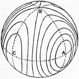
Fig. 80.

The signs of the coefficients follow the same rule as in the case of (4). The possible forms of the invariable cone are indicated in fig. 80 by means of the intersections with a concentric spherical surface. In the critical case of 2BT = Γ2 the cone degenerates into two planes. It appears that if the body be sightly disturbed from a state of rotation about the principal axis of greatest or least moment, the invariable cone will closely surround this axis, which will therefore never deviate far from the invariable line. If, on the other hand, the body be slightly disturbed from a state of rotation about the mean axis a wide deviation will take place. Hence a rotation about the axis of greatest or least moment is reckoned as stable, a rotation about the mean axis as unstable. The question is greatly simplified when two of the principal moments are equal, say A = B. The polhode and herpolhode cones are then right circular, and the motion is “precessional” according to the definition of § 18. If α be the inclination of the instantaneous axis to the axis of symmetry, β the inclination of the latter axis to the invariable line, we have

Γ cos β = C ω cos α, Γ sin β = A ω sin α,

(6)

whence

tan β A tan α.

C

(7)

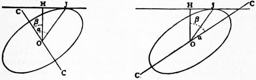
Fig. 81.

Hence β ≷ α, and the circumstances are therefore those of the first or second case in fig. 78, according as A ≷ C. If ψ be the rate at which the plane HOJ revolves about OH, we have

ψ = sin α ω = C cos α ω,

sin β A cos β

(8)

by § 18 (3). Also if χ̇ be the rate at which J describes the polhode, we have ψ̇ sin (β − α) = χ̇ sin β, whence

χ̇ = sin (α − β) ω.

sin α

(9)

If the instantaneous axis only deviate slightly from the axis of symmetry the angles α, β are small, and χ̇ = (A − C) A·ω; the instantaneous axis therefore completes its revolution in the body in the period

2π = A − C ω.

χ̇ A

(10)

In the case of the earth it is inferred from the independent phenomenon of luni-solar precession that (C − A)/A = .00313. Hence if the earth’s axis of rotation deviates slightly from the axis of figure, it should describe a cone about the latter in 320 sidereal days. This would cause a periodic variation in the latitude of any place on the earth’s surface, as determined by astronomical methods. There appears to be evidence of a slight periodic variation of latitude, but the period would seem to be about fourteen months. The discrepancy is attributed to a defect of rigidity in the earth. The phenomenon is known as the Eulerian nutation, since it is supposed to come under the free rotations first discussed by Euler.

§ 20. Motion of a Solid of Revolution.—In the case of a solid of revolution, or (more generally) whenever there is kinetic symmetry about an axis through the mass-centre, or through a fixed point O, a number of interesting problems can be treated almost directly from first principles. It frequently happens that the extraneous forces have zero moment about the axis of symmetry, as e.g. in the case of the flywheel of a gyroscope if we neglect the friction at the bearings. The angular velocity (r) about this axis is then constant. For we have seen that r is constant when there are no extraneous forces; and r is evidently not affected by an instantaneous impulse which leaves the angular momentum Cr, about the axis of symmetry, unaltered. And a continuous force may be regarded as the limit of a succession of infinitesimal instantaneous impulses.

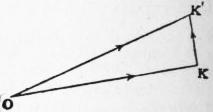
Fig. 82.

Suppose, for example, that a flywheel is rotating with angular velocity n about its axis, which is (say) horizontal, and that this axis is made to rotate with the angular velocity ψ̇ in the horizontal plane. The components of angular momentum about the axis of the flywheel and about the vertical will be Cn and A ψ̇ respectively, where A is the moment of inertia about any axis through the mass-centre (or through the fixed point O) perpendicular to that of symmetry. If OK> be the vector representing the former component at time t, the vector which represents it at time t + δt will be OK′>, equal to OK> in magnitude and making with it an angle δψ. Hence KK′> (= Cn δψ) will represent the change in this component due to the extraneous forces. Hence, so far as this component is concerned, the extraneous forces must supply a couple of moment Cnψ̇ in a vertical plane through the axis of the flywheel. If this couple be absent, the axis will be tilted out of the horizontal plane in such a sense that the direction of the spin n approximates to that of the azimuthal rotation ψ̇. The remaining constituent of the extraneous forces is a couple Aψ̈ about the vertical; this vanishes if ψ̇ is constant. If the axis of the flywheel make an angle θ with the vertical, it is seen in like manner that the required couple in the vertical plane through the axis is Cn sin θ ψ̇. This matter can be strikingly illustrated with an ordinary gyroscope, e.g. by making the larger movable ring in fig. 37 rotate about its vertical diameter.

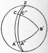
Fig. 83.

If the direction of the axis of kinetic symmetry be specified by means of the angular co-ordinates θ, ψ of § 7, then considering the component velocities of the point C in fig. 83, which are θ̇ and sin θψ̇ along and perpendicular to the meridian ZC, we see that the component angular velocities about the lines OA′, OB′ are −sin θ ψ̇ and θ̇ respectively. Hence if the principal moments of inertia at O be A, A, C, and if n be the constant angular velocity about the axis OC, the kinetic energy is given by

2T = A (θ̇2 + sin2 θψ̇2) + Cn2.

(1)

Again, the components of angular momentum about OC, OA′ are Cn, −A sin θ ψ̇, and therefore the angular momentum (μ, say) about OZ is

μ = A sin2 θψ̇ + Cn cos θ.

(2)

We can hence deduce the condition of steady precessional motion in a top. A solid of revolution is supposed to be free to turn about a fixed point O on its axis of symmetry, its mass-centre G being in this axis at a distance h from O. In fig. 83 OZ is supposed to be vertical, and OC is the axis of the solid drawn in the direction OG. If θ is constant the points C, A′ will in time δt come to positions C″, A″ such that CC″ = sin θ δψ, A′A″ = cos θ δψ, and the angular momentum about OB′ will become Cn sin θ δψ − A sin θ ψ̇ · cos θ δψ. Equating this to Mgh sin θ δt, and dividing out by sin θ, we obtain

A cos θ ψ̇2 − Cnψ̇ + Mgh = 0,

(3)

as the condition in question. For given values of n and θ we have two possible values of ψ̇ provided n exceed a certain limit. With a very rapid spin, or (more precisely) with Cn large in comparison with √(4AMgh cos θ), one value of ψ̇ is small and the other large, viz. the two values are Mgh/Cn and Cn/A cos θ approximately. The absence of g from the latter expression indicates that the circumstances of the rapid precession are very nearly those of a free Eulerian rotation (§ 19), gravity playing only a subordinate part.

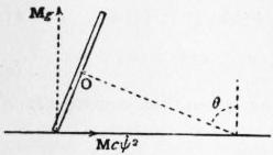
Fig. 84.

Again, take the case of a circular disk rolling in steady motion on a horizontal plane. The centre O of the disk is supposed to describe a horizontal circle of radius c with the constant angular velocity ψ̇, whilst its plane preserves a constant inclination θ to the horizontal. The components of the reaction of the horizontal lane will be Mcψ̇2 at right angles to the tangent line at the point of contact and Mg vertically upwards, and the moment of these about the horizontal diameter of the disk, which corresponds to OB′ in fig. 83, is Mcψ̇2. α sin θ − Mgα cos θ, where α is the radius of the disk. Equating this to the rate of increase of the angular momentum about OB′, investigated as above, we find

( C + Ma2 + A a cos θ ) ψ̇2 = Mg a2 cot θ,

c c

(4)

where use has been made of the obvious relation nα = cψ̇. If c and θ be given this formula determines the value of ψ̇ for which the motion will be steady.

In the case of the top, the equation of energy and the condition of constant angular momentum (μ) about the vertical OZ are sufficient to determine the motion of the axis. Thus, we have

1⁄2A (θ̇2 + sin2 θψ̇2) + 1⁄2Cn2 + Mgh cos θ = const.,

(5)

A sin2 θψ̇ + ν cos θ = μ,

(6)

where ν is written for Cn. From these ψ̇ may be eliminated, and on differentiating the resulting equation with respect to t we obtain

Aθ̈ − (μ − ν cos θ) (μ cos θ − ν) − Mgh sin θ = 0.

A sin3 θ

(7)

If we put θ̈ = 0 we get the condition of steady precessional motion in a form equivalent to (3). To find the small oscillation about a state of steady precession in which the axis makes a constant angle α with the vertical, we write θ = α + χ, and neglect terms of the second order in χ. The result is of the form

χ̈ + σ2χ = 0,

(8)

where

σ2 = { (μ − ν cos α)2 + 2 (μ − ν cos α) (μ cos α − ν) cos α + (μ cos α − ν)2 } / A2 sin4 α.

(9)

When ν is large we have, for the “slow” precession σ = ν/A, and for the “rapid” precession σ = A/ν cos α = ψ̇, approximately. Further, on examining the small variation in ψ̇, it appears that in a slightly disturbed slow precession the motion of any point of the axis consists of a rapid circular vibration superposed on the steady precession, so that the resultant path has a trochoidal character. This is a type of motion commonly observed in a top spun in the ordinary way, although the successive undulations of the trochoid may be too small to be easily observed. In a slightly disturbed rapid precession the superposed vibration is elliptic-harmonic, with a period equal to that of the precession itself. The ratio of the axes of the ellipse is sec α, the longer axis being in the plane of θ. The result is that the axis of the top describes a circular cone about a fixed line making a small angle with the vertical. This is, in fact, the “invariable line” of the free Eulerian rotation with which (as already remarked) we are here virtually concerned. For the more general discussion of the motion of a top see Gyroscope.