VOLUME XVII SLICE VIII Matter to Mecklenburg (continued 10)

§ 21. Moving Axes of Reference.—For the more general treatment of the kinetics of a rigid body it is usually convenient to adopt a system of moving axes. In order that the moments and products of inertia with respect to these axes may be constant, it is in general necessary to suppose them fixed in the solid.

We will assume for the present that the origin O is fixed. The moving axes Ox, Oy, Oz form a rigid frame of reference whose motion at time t may be specified by the three component angular velocities p, q, r. The components of angular momentum about Ox, Oy, Oz will be denoted as usual by λ, μ, ν. Now consider a system of fixed axes Ox′, Oy′, Oz′ chosen so as to coincide at the instant t with the moving system Ox, Oy, Oz. At the instant t + δt, Ox, Oy, Oz will no longer coincide with Ox′, Oy′, Oz′; in particular they will make with Ox′ angles whose cosines are, to the first order, 1, −rδt, qδt, respectively. Hence the altered angular momentum about Ox′ will be λ + δλ + (μ + δμ) (−rδt) + (ν + δν) qδt. If L, M, N be the moments of the extraneous forces about Ox, Oy, Oz this must be equal to λ + Lδt. Hence, and by symmetry, we obtain

dλ − rν + qν = L,

dt

dμ − pν + rλ = M,

dt

dν − qλ + pν = N.

dt

(1)

These equations are applicable to any dynamical system whatever. If we now apply them to the case of a rigid body moving about a fixed point O, and make Ox, Oy, Oz coincide with the principal axes of inertia at O, we have λ, μ, ν = Ap, Bq, Cr, whence

A dp − (B − C) qr = L,

dt

B dq − (C − A) rp = M,

C dr − (A − B) pq = N.

dt

(2)

If we multiply these by p, q, r and add, we get

d · 1⁄2 (Ap2 + Bq2 + Cr2) = Lp + Mq + Nr,

dt

(3)

which is (virtually) the equation of energy.

As a first application of the equations (2) take the case of a solid constrained to rotate with constant angular velocity ω about a fixed axis (l, m, n). Since p, q, r are then constant, the requisite constraining couple is

L = (C − B) mnω2, M = (A − C) nlω2, N = (B − A) lmω2.

(4)

If we reverse the signs, we get the “centrifugal couple” exerted by the solid on its bearings. This couple vanishes when the axis of rotation is a principal axis at O, and in no other case (cf. § 17).

If in (2) we put, L, M, N = O we get the case of free rotation; thus

A dp (B − C) qr,

dt

B dq (C − A) rp,

dt

C dr (A − B) pq.

dt

(5)

These equations are due to Euler, with whom the conception of moving axes, and the application to the problem of free rotation, originated. If we multiply them by p, q, r, respectively, or again by Ap, Bq, Cr respectively, and add, we verify that the expressions Ap2 + Bq2 + Cr2 and A2p2 + B2q2 + C2r2 are both constant. The former is, in fact, equal to 2T, and the latter to Γ2, where T is the kinetic energy and Γ the resultant angular momentum.

To complete the solution of (2) a third integral is required; this involves in general the use of elliptic functions. The problem has been the subject of numerous memoirs; we will here notice only the form of solution given by Rueb (1834), and at a later period by G. Kirchhoff (1875), If we write

u = ∫φ0 dφ , Δφ = √(1 − k2 sin2 φ),

Δφ

we have, in the notation of elliptic functions, φ = am u. If we assume

p = p0 cos am (σt + ε), q = q0sin am (σt + ε), r = r0Δ am (σt + ε),

(7)

we find

ṗ = − σp0 qr, q̇ = σq0 rp, ṙ = k2σr0 pq.

q0r0 r0p0 p0q0

(8)

Hence (5) will be satisfied, provided

−σp0 = B − C , σq0 = C − A , −k2σr0 = A − B .

q0r0 A r0p0 B p0q0 C

(9)

These equations, together with the arbitrary initial values of p, q, r, determine the six constants which we have denoted by p0, q0, r0, k2, σ, ε. We will suppose that A > B > C. From the form of the polhode curves referred to in § 19 it appears that the angular velocity q about the axis of mean moment must vanish periodically. If we adopt one of these epochs as the origin of t, we have ε = 0, and p0, r0 will become identical with the initial values of p, r. The conditions (9) then lead to

q02 = A (A − C) p02, σ2 = (A − C) (B − C) r02, k2 = A (A − B) · p02 .

B (B − C) AB C (B − C) r02

(10)

For a real solution we must have k2 < 1, which is equivalent to 2BT > Γ2. If the initial conditions are such as to make 2BT < Γ2, we must interchange the forms of p and r in (7). In the present case the instantaneous axis returns to its initial position in the body whenever φ increases by 2π, i.e. whenever t increases by 4K/σ, when K is the “complete” elliptic integral of the first kind with respect to the modulus k.

The elliptic functions degenerate into simpler forms when k2 = 0 or k2 = 1. The former case arises when two of the principal moments are equal; this has been sufficiently dealt with in § 19. If k2 = 1, we must have 2BT = Γ2. We have seen that the alternative 2BT ≷ Γ2 determines whether the polhode cone surrounds the principal axis of least or greatest moment. The case of 2BT = Γ2, exactly, is therefore a critical case; it may be shown that the instantaneous axis either coincides permanently with the axis of mean moment or approaches it asymptotically.

When the origin of the moving axes is also in motion with a velocity whose components are u, v, w, the dynamical equations are

dξ − rη + qζ = X, dη − pζ + rχ = Y, dζ − qχ + pη = Z,

dt dt dt

(11)

dλ − rμ + qν − wη + vζ = L, dμ − pν + rλ- uζ + wξ = M,

dt dt

dν − qλ + pμ − vξ + uη = N.

dt

(12)

To prove these, we may take fixed axes O′x′, O′y′, O′z′ coincident with the moving axes at time t, and compare the linear and angular momenta ξ + δξ, η + δη, ζ + δζ, λ + δλ, μ + δμ, ν + δν relative to the new position of the axes, Ox, Oy, Oz at time t + δt with the original momenta ξ, η, ζ, λ, μ, ν relative to O′x′, O′y′, O′z′ at time t. As in the case of (2), the equations are applicable to any dynamical system whatever. If the moving origin coincide always with the mass-centre, we have ξ, η, ζ = M0u, M0v, M0w, where M0 is the total mass, and the equations simplify.

When, in any problem, the values of u, v, w, p, q, r have been determined as functions of t, it still remains to connect the moving axes with some fixed frame of reference. It will be sufficient to take the case of motion about a fixed point O; the angular co-ordinates θ, φ, ψ of Euler may then be used for the purpose. Referring to fig. 36 we see that the angular velocities p, q, r of the moving lines, OA, OB, OC about their instantaneous positions are

p = θ̇ sin φ − sin θ cos φψ̇, q = θ̇ cos φ + sin θ sin φψ̇, r = φ̇ + cos θψ̇,

(13)

by § 7 (3), (4). If OA, OB, OC be principal axes of inertia of a solid, and if A, B, C denote the corresponding moments of inertia, the kinetic energy is given by

2T = A (θ̇ sin φ − sin θ cos φψ̇)2 + B (θ̇ cos φ + sin θ sin θψ)2 + C (φ̇ + cos θψ̇)2.

(14)

If A = B this reduces to

2T = A (θ̇2 + sin2 θ ψ̇2) + C (φ̇ + cos θ ψ̇)2;

(15)

cf. § 20 (1).

§ 22. Equations of Motion in Generalized Co-ordinates.—Suppose we have a dynamical system composed of a finite number of material particles or rigid bodies, whether free or constrained in any way, which are subject to mutual forces and also to the action of any given extraneous forces. The configuration of such a system can be completely specified by means of a certain number (n) of independent quantities, called the generalized co-ordinates of the system. These co-ordinates may be chosen in an endless variety of ways, but their number is determinate, and expresses the number of degrees of freedom of the system. We denote these co-ordinates by q1, q2, ... qn. It is implied in the above description of the system that the Cartesian co-ordinates x, y, z of any particle of the system are known functions of the q’s, varying in form (of course) from particle to particle. Hence the kinetic energy T is given by

2T = Σ {m (ẋ2 + ẏ2 + ż2) }

= a11q̇12 + a22q̇22 + ... + 2a12q̇1q̇2 + ...,

(1)

where

arr = Σ [ m { ( ∂x )2 + ( ∂y )2 + ( ∂z )2 } ],

∂qr ∂qr ∂qr

ars = Σ { m ( ∂x ∂x + ∂y ∂y + ∂z ∂z ) } = asr.

∂qr ∂qs ∂qr ∂qs ∂qr ∂qs

(2)

Thus T is expressed as a homogeneous quadratic function of the quantities q̇1, q̇2, ... q̇n, which are called the generalized components of velocity. The coefficients arr, ars are called the coefficients of inertia; they are not in general constants, being functions of the q’s and so variable with the configuration. Again, If (X, Y, Z) be the force on m, the work done in an infinitesimal change of configuration is

Σ (Xδx + Yδy + Zδz) = Q1δq1 + Q2δq2 + ... + Qnδqn,

(3)

where

Qr = Σ ( X ∂x + Y ∂y + Z ∂z ).

∂qr ∂qr ∂qr

(4)

The quantities Qr are called the generalized components of force.

The equations of motion of m being

mẍ = X, mÿ = Y, mz̈ = Z,

(5)

we have

Σ { m ( ẍ ∂x + ÿ ∂y + z̈ ∂z ) } = Qr.

∂qr ∂qr ∂qr

(6)

Now

(7)

ẋ = ∂x q̇1 + ∂x q̇2 + ... + ∂x q̇n,

∂q1 ∂q2 ∂qn

whence

(8)

∂ẋ = ∂x .

∂q̇r ∂qr

Also

(9)

d ( ∂x ) = ∂2x q̇1 + ∂2x q̇2 + ... + ∂2x q̇r = ∂ẋ .

dt ∂qr ∂q1∂qr ∂q2∂qr ∂qn∂qr ∂qr

Hence

(10)

ẍ ∂x = d ( ẋ ∂x ) − ẋ d ( ∂x ) = d ( ẋ ∂ẋ ) − ẋ ∂ẋ .

∂qr dt ∂qr dt ∂qr dt ∂q̇r ∂qr

By these and the similar transformations relating to y and z the equation (6) takes the form

d ( ∂T ) − ∂T = Qr.

dt ∂q̇r ∂qr

(11)

If we put r = 1, 2, ... n in succession, we get the n independent equations of motion of the system. These equations are due to Lagrange, with whom indeed the first conception, as well as the establishment, of a general dynamical method applicable to all systems whatever appears to have originated. The above proof was given by Sir W. R. Hamilton (1835). Lagrange’s own proof will be found under Dynamics, § Analytical. In a conservative system free from extraneous force we have

Σ (X δx + Y δy + Z δz) = −δV,

(12)

where V is the potential energy. Hence

Qr = − ∂V ,

∂qr

(13)

and

d ( ∂T ) − ∂T = − ∂V .

dt ∂q̇r ∂qr ∂qr

(14)

If we imagine any given state of motion (q̇1, q̇2 ... q̇n) through the configuration (q1, q2, ... qn) to be generated instantaneously from rest by the action of suitable impulsive forces, we find on integrating (11) with respect to t over the infinitely short duration of the impulse

∂T = Qr′,

∂q̇r

(15)

where Qr′ is the time integral of Qr and so represents a generalized component of impulse. By an obvious analogy, the expressions ∂T/∂q̇r may be called the generalized components of momentum; they are usually denoted by pr thus

pr = ∂T / ∂q̇r = a1rq̇1 + a2rq̇2 + ... + anrq̇n.

(16)

Since T is a homogeneous quadratic function of the velocities q̇1, q̇2, ... q̇n, we have

2T = ∂T q̇1 + ∂T q̇2 + ... + ∂T q̇n = p1q̇2 + p2q̇2 + ... + pnq̇n.

∂q̇1 ∂q̇2 ∂q̇n

(17)

Hence

2 dT = ṗ1q̇1 + ṗ2q̇2 + ... + ṗnq̇n + ṗ1q̈1 + ṗ2q̈2 + ... + ṗnq̈n

dt

= ( ∂T + Q1 ) q̇1 + ( ∂T + Q2 ) q̇2 + ... + ( ∂T + Qn ) q̇n + ∂T q̈1 + ∂T q̈2 + ... + ∂T q̈n

∂q̇1 ∂q̇2 ∂q̇n ∂q̇1 ∂q̇2 ∂q̇n

= dT + Q1q̇1 + Q2q̇2 + ... + Qnq̇n,

dt

(18)

or

dT = Q1q̇1 + Q2q̇2 + ... + Qnq̇n.

dt

(19)

This equation expresses that the kinetic energy is increasing at a rate equal to that at which work is being done by the forces. In the case of a conservative system free from extraneous force it becomes the equation of energy

d (T + V) = 0, or T + V = const.,

dt

(20)

in virtue of (13).

As a first application of Lagrange’s formula (11) we may form the equations of motion of a particle in spherical polar co-ordinates. Let r be the distance of a point P from a fixed origin O, θ the angle which OP makes with a fixed direction OZ, ψ the azimuth of the plane ZOP relative to some fixed plane through OZ. The displacements of P due to small variations of these co-ordinates are ∂r along OP, r δθ perpendicular to OP in the plane ZOP, and r sin θ δψ perpendicular to this plane. The component velocities in these directions are therefore ṙ, rθ̇, r sin θψ̇, and if m be the mass of a moving particle at P we have

2T = m (ṙ2 + r2θ;̇2 + r2 sin2 θψ;̇2).

(21)

Hence the formula (11) gives

m (r̈ − rθ̇2 − r sin2 θψ̇2) = R,

d/dt (mr2θ̇) − mr2 · sin θ cos θψ̇2 = Θ,

d/dt (mr2 sin2 θψ̇) = Ψ.

(22)

The quantities R, Θ, Ψ are the coefficients in the expression R δr + Θ δθ + Ψ δψ for the work done in an infinitely small displacement; viz. R is the radial component of force, Θ is the moment about a line through O perpendicular to the plane ZOP, and Ψ is the moment about OZ. In the case of the spherical pendulum we have r = l, Θ = − mgl sin θ, Ψ = 0, if OZ be drawn vertically downwards, and therefore

θ̈ − sin θ cos θψ̇2 = − (g/l) sin θ,

sin2 θψ̇ = h,

(23)

where h is a constant. The latter equation expresses that the angular momentum ml2 sin2 θψ̇ about the vertical OZ is constant. By elimination of ψ̇ we obtain

θ̈ − h2 cos2 θ / sin3 θ = − g sin θ.

l

(24)

If the particle describes a horizontal circle of angular radius α with constant angular velocity Ω, we have ω̇ = 0, h = Ω2 sin α, and therefore

Ω2 = g cos α,

l

(25)

as is otherwise evident from the elementary theory of uniform circular motion. To investigate the small oscillations about this state of steady motion we write θ = α + χ in (24) and neglect terms of the second order in χ. We find, after some reductions,

χ̈ + (1 + 3 cos2 α) Ω2χ = 0;

(26)

this shows that the variation of χ is simple-harmonic, with the period

2π / √(1 + 3 cos2 α)·Ω

As regards the most general motion of a spherical pendulum, it is obvious that a particle moving under gravity on a smooth sphere cannot pass through the highest or lowest point unless it describes a vertical circle. In all other cases there must be an upper and a lower limit to the altitude. Again, a vertical plane passing through O and a point where the motion is horizontal is evidently a plane of symmetry as regards the path. Hence the path will be confined between two horizontal circles which it touches alternately, and the direction of motion is never horizontal except at these circles. In the case of disturbed steady motion, just considered, these circles are nearly coincident. When both are near the lowest point the horizontal projection of the path is approximately an ellipse, as shown in § 13; a closer investigation shows that the ellipse is to be regarded as revolving about its centre with the angular velocity 2⁄3 abΩ/l2, where a, b are the semi-axes.

To apply the equations (11) to the case of the top we start with the expression (15) of § 21 for the kinetic energy, the simplified form (1) of § 20 being for the present purpose inadmissible, since it is essential that the generalized co-ordinates employed should be competent to specify the position of every particle. If λ, μ, ν be the components of momentum, we have

λ = ∂T / ∂θ̇ = Aθ̇,

μ = ∂T / ∂ψ̇ = A sin2 θψ̇ + C (φ̇ + cos θψ̇) cos θ,

ν = ∂T / ∂φ̇ = C (θ̇ + cos θψ̇).

(27)

The meaning of these quantities is easily recognized; thus λ is the angular momentum about a horizontal axis normal to the plane of θ, μ is the angular momentum about the vertical OZ, and ν is the angular momentum about the axis of symmetry. If M be the total mass, the potential energy is V = Mgh cos θ, if OZ be drawn vertically upwards. Hence the equations (11) become

Aθ̇ − A sin θ cos θψ̇2 + C (φ̇ + cos θψ̇) ψ̇ sin θ = Mgh sin θ,

d/dt · { A sin2 θψ̇ + C(φ̇ + cos θψ̇) cos θ } = 0,

d/dt · { C (φ̇ + cos θψ̇) } = 0,

(28)

of which the last two express the constancy of the momenta μ, ν. Hence

Aθ̈ − A sin θ cos θψ̇2 + ν sin θψ̇ = Mgh sin θ, A sin2 θψ̇ + ν cosθ = μ.

(29)

If we eliminate ψ̇ we obtain the equation (7) of § 20. The theory of disturbed precessional motion there outlined does not give a convenient view of the oscillations of the axis about the vertical position. If θ be small the equations (29) may be written

θ̈ − θω̇2 = − ν2 − 4AMgh θ,

4A2

θ2ω̇ = const.,

(30)

where

ω = ψ − ν t.

2A

(31)

Since θ, ω are the polar co-ordinates (in a horizontal plane) of a point on the axis of symmetry, relative to an initial line which revolves with constant angular velocity ν/2A, we see by comparison with § 14 (15) (16) that the motion of such a point will be elliptic-harmonic superposed on a uniform rotation ν/2A, provided ν2 > 4AMgh. This gives (in essentials) the theory of the “gyroscopic pendulum.”

§ 23. Stability of Equilibrium. Theory of Vibrations.—If, in a conservative system, the configuration (q1, q2, ... qn) be one of equilibrium, the equations (14) of § 22 must be satisfied by q̇1, q̇2 ... q̇n = 0, whence

∂V / ∂qr = 0.

(1)

A necessary and sufficient condition of equilibrium is therefore that the value of the potential energy should be stationary for infinitesimal variations of the co-ordinates. If, further, V be a minimum, the equilibrium is necessarily stable, as was shown by P. G. L. Dirichlet (1846). In the motion consequent on any slight disturbance the total energy T + V is constant, and since T is essentially positive it follows that V can never exceed its equilibrium value by more than a slight amount, depending on the energy of the disturbance. This implies, on the present hypothesis, that there is an upper limit to the deviation of each co-ordinate from its equilibrium value; moreover, this limit diminishes indefinitely with the energy of the original disturbance. No such simple proof is available to show without qualification that the above condition is necessary. If, however, we recognize the existence of dissipative forces called into play by any motion whatever of the system, the conclusion can be drawn as follows. However slight these forces may be, the total energy T + V must continually diminish so long as the velocities q̇1, q̇2, ... q̇n differ from zero. Hence if the system be started from rest in a configuration for which V is less than in the equilibrium configuration considered, this quantity must still further decrease (since T cannot be negative), and it is evident that either the system will finally come to rest in some other equilibrium configuration, or V will in the long run diminish indefinitely. This argument is due to Lord Kelvin and P. G. Tait (1879).

In discussing the small oscillations of a system about a configuration of stable equilibrium it is convenient so to choose the generalized cc-ordinates q1, q2, ... qn that they shall vanish in the configuration in question. The potential energy is then given with sufficient approximation by an expression of the form

2V = c11q12 + c22q22 + ... + 2c12q1q2 + ...,

(2)

a constant term being irrelevant, and the terms of the first order being absent since the equilibrium value of V is stationary. The coefficients crr, crs are called coefficients of stability. We may further treat the coefficients of inertia arr, ars of § 22 (1) as constants. The Lagrangian equations of motion are then of the type

a1rq̈1 + a2rq̈2 + ... + anrq̈n + c1rq1 + c2rq2 + ... + cnrqn = Qr,

(3)

where Qr now stands for a component of extraneous force. In a free oscillation we have Q1, Q2, ... Qn = 0, and if we assume

qr = Ar eiσt,

(4)

we obtain n equations of the type

(c1r − σ2a1r) A1 + (c2r − σ2a2r) A2 + ... + (cnr − σ2anr) An = 0.

(5)

Eliminating the n − 1 ratios A1 : A2 : ... : An we obtain the determinantal equation

Δ (σ2) = 0,

(6)

where

Δ(σ2) = c11 − σ2a11, c21 − σ2a21, ..., Cn1 − σ2anl

c12 − σ2a12, c22 − σ2a22, ..., Cn2 − σ2an2

. . ... .

. . ... .

. . ... .

c1n − σ2a1n, c2n − σ2a2n, ..., Cnn − σ2ann

(7)

The quadratic expression for T is essentially positive, and the same holds with regard to V in virtue of the assumed stability. It may be shown algebraically that under these conditions the n roots of the above equation in σ2 are all real and positive. For any particular root, the equations (5) determine the ratios of the quantities A1, A2, ... An, the absolute values being alone arbitrary; these quantities are in fact proportional to the minors of any one row in the determinate Δ(σ2). By combining the solutions corresponding to a pair of equal and opposite values of σ we obtain a solution in real form:

qr = Car cos (σt + ε),

(8)

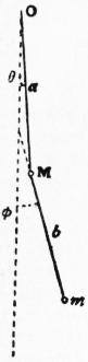
Fig. 85.

where a1, a2 ... ar are a determinate series of quantities having to one another the above-mentioned ratios, whilst the constants C, ε are arbitrary. This solution, taken by itself, represents a motion in which each particle of the system (since its displacements parallel to Cartesian co-ordinate axes are linear functions of the q’s) executes a simple vibration of period 2π/σ. The amplitudes of oscillation of the various particles have definite ratios to one another, and the phases are in agreement, the absolute amplitude (depending on C) and the phase-constant (ε) being alone arbitrary. A vibration of this character is called a normal mode of vibration of the system; the number n of such modes is equal to that of the degrees of freedom possessed by the system. These statements require some modification when two or more of the roots of the equation (6) are equal. In the case of a multiple root the minors of Δ(σ2) all vanish, and the basis for the determination of the quantities ar disappears. Two or more normal modes then become to some extent indeterminate, and elliptic vibrations of the individual particles are possible. An example is furnished by the spherical pendulum (§ 13).

As an example of the method of determination of the normal modes we may take the “double pendulum.” A mass M hangs from a fixed point by a string of length a, and a second mass m hangs from M by a string of length b. For simplicity we will suppose that the motion is confined to one vertical plane. If θ, φ be the inclinations of the two strings to the vertical, we have, approximately,

2T = Ma2θ̇2 + m (aθ̇ + bψ̇)2

2V = Mgaθ2 + mg (aθ2 + bψ2).

(9)

The equations (3) take the forms

aθ ̈ + μbφ̈ + gθ = 0,

aθ ̈ + bφ̈ + gφ = 0.

(10)

where μ = m/(M + m). Hence

(σ2 − g/a) aθ + μσ2bφ = 0,

σ2aθ + (σ2 − g/b) bφ = 0.

(11)

The frequency equation is therefore

(σ2 − g/a) (σ2 − g/b) − μσ4 = 0.

(12)

The roots of this quadratic in σ2 are easily seen to be real and positive. If M be large compared with m, μ is small, and the roots are g/a and g/b, approximately. In the normal mode corresponding to the former root, M swings almost like the bob of a simple pendulum of length a, being comparatively uninfluenced by the presence of m, whilst m executes a “forced” vibration (§ 12) of the corresponding period. In the second mode, M is nearly at rest [as appears from the second of equations (11)], whilst m swings almost like the bob of a simple pendulum of length b. Whatever the ratio M/m, the two values of σ2 can never be exactly equal, but they are approximately equal if a, b are nearly equal and μ is very small. A curious phenomenon is then to be observed; the motion of each particle, being made up (in general) of two superposed simple vibrations of nearly equal period, is seen to fluctuate greatly in extent, and if the amplitudes be equal we have periods of approximate rest, as in the case of “beats” in acoustics. The vibration then appears to be transferred alternately from m to M at regular intervals. If, on the other hand, M is small compared with m, μ is nearly equal to unity, and the roots of (12) are σ2 = g/(a + b) and σ2 = mg/M·(a + b)/ab, approximately. The former root makes θ = φ, nearly; in the corresponding normal mode m oscillates like the bob of a simple pendulum of length a + b. In the second mode aθ + bφ = 0, nearly, so that m is approximately at rest. The oscillation of M then resembles that of a particle at a distance a from one end of a string of length a + b fixed at the ends and subject to a tension mg.

The motion of the system consequent on arbitrary initial conditions may be obtained by superposition of the n normal modes with suitable amplitudes and phases. We have then

qr = αrθ + αr′θ′ + αr″θ″ + ...,

(13)

where

θ = C cos (σt + ε), θ′ = C′ cos (σ′t + ε), θ″ = C″ cos (σ″t + ε), ...

(14)

provided σ2, σ′2, σ″2, ... are the n roots of (6). The coefficients of θ, θ′, θ″, ... in (13) satisfy the conjugate or orthogonal relations

a11α1α1′ + a22α2α2′ + ... + a12 (α1α2′ + α2α1′) + ... = 0,

(15)

c11α1α1′ + c22α2α2′ + ... + c12 (α1α2′ + α2α1′) + ... = 0,

(16)

provided the symbols αr, αr′ correspond to two distinct roots σ2, σ′2 of (6). To prove these relations, we replace the symbols A1, A2, ... An in (5) by α1, α2, ... αn respectively, multiply the resulting equations by a′1, a′2, ... a′n, in order, and add. The result, owing to its symmetry, must still hold if we interchange accented and unaccented Greek letters, and by comparison we deduce (15) and (16), provided σ2 and σ′2 are unequal. The actual determination of C, C′, C″, ... and ε, ε′, ε″, ... in terms of the initial conditions is as follows. If we write

C cos ε = H, −C sin ε = K,

(17)

we must have

αrH + αr′H′ + αr″H″ + ... = [qr]0,

σαrH + σ′αr′H′ + σ″αr″H″ + ... = [q̇r]0,

(18)

where the zero suffix indicates initial values. These equations can be at once solved for H, H′, H″, ... and K, K′, K″, ... by means of the orthogonal relations (15).

By a suitable choice of the generalized co-ordinates it is possible to reduce T and V simultaneously to sums of squares. The transformation is in fact effected by the assumption (13), in virtue of the relations (15) (16), and we may write

2T = aθ̇2 + a′θ̇′2 + a″θ̇″2 + ..., 2V = cθ2 + c′θ′2 + c″θ″2 + ....

(19)

The new co-ordinates θ, θ′, θ″ ... are called the normal co-ordinates of the system; in a normal mode of vibration one of these varies alone. The physical characteristics of a normal mode are that an impulse of a particular normal type generates an initial velocity of that type only, and that a constant extraneous force of a particular normal type maintains a displacement of that type only. The normal modes are further distinguished by an important “stationary” property, as regards the frequency. If we imagine the system reduced by frictionless constraints to one degree of freedom, so that the co-ordinates θ, θ′, θ″, ... have prescribed ratios to one another, we have, from (19),

σ2 = cθ2 + c′θ′2 = c″θ″2 + ... ,

aθ2 + a′θ′2 + a″θ″2 + ...

(20)

This shows that the value of σ2 for the constrained mode is intermediate to the greatest and least of the values c/a, c′/a′, c″/a″, ... proper to the several normal modes. Also that if the constrained mode differs little from a normal mode of free vibration (e.g. if θ′, θ″, ... are small compared with θ), the change in the frequency is of the second order. This property can often be utilized to estimate the frequency of the gravest normal mode of a system, by means of an assumed approximate type, when the exact determination would be difficult. It also appears that an estimate thus obtained is necessarily too high.

From another point of view it is easily recognized that the equations (5) are exactly those to which we are led in the ordinary process of finding the stationary values of the function

V (q1, q2, ... qn) ,

T (q1, q2, ... qn)

where the denominator stands for the same homogeneous quadratic function of the q’s that T is for the q̇’s. It is easy to construct in this connexion a proof that the n values of σ2 are all real and positive.

The case of three degrees of freedom is instructive on account of the geometrical analogies. With a view to these we may write

2T = aẋ2 + bẏ2 + cż2 + 2fẏż + 2gżẋ + 2hẋẏ,

2V = Ax2 + By2 + Cz2 + 2Fyz + 2Gzx + 2Hxy.

(21)

It is obvious that the ratio

V (x, y, z)

T (x, y, z)

(22)

must have a least value, which is moreover positive, since the numerator and denominator are both essentially positive. Denoting this value by σ12, we have

Ax1 + Hy1 + Gz1 = σ12 (ax1 + hy1 + ∂gz1),

Hx1 + By1 + Fz1 = σ12 (hx1 + by1 + fz1),

Gx1 + Fy1 + Cz1 = σ12 (gx1 + fy1 + cz1),

(23)

provided x1 : y1 : z1 be the corresponding values of the ratios x:y:z. Again, the expression (22) will also have a least value when the ratios x : y : z are subject to the condition

x1 ∂V + y1 ∂V + z1 ∂V = 0;

∂x ∂y ∂z

(24)

and if this be denoted by σ22 we have a second system of equations similar to (23). The remaining value σ22 is the value of (22) when x : y : z arc chosen so as to satisfy (24) and

x2 ∂V + y2 ∂V + z2 ∂V = 0;

∂x ∂y ∂z

(25)

The problem is identical with that of finding the common conjugate diameters of the ellipsoids T(x, y, z) = const., V(x, y, z) = const. If in (21) we imagine that x, y, z denote infinitesimal rotations of a solid free to turn about a fixed point in a given field of force, it appears that the three normal modes consist each of a rotation about one of the three diameters aforesaid, and that the values of σ are proportional to the ratios of the lengths of corresponding diameters of the two quadrics.

We proceed to the forced vibrations of the system. The typical case is where the extraneous forces are of the simple-harmonic type cos (σt + ε); the most general law of variation with time can be derived from this by superposition, in virtue of Fourier’s theorem. Analytically, it is convenient to put Qr, equal to eiσt multiplied by a complex coefficient; owing to the linearity of the equations the factor eiσt will run through them all, and need not always be exhibited. For a system of one degree of freedom we have

aq̈ + cq = Q,

(26)

and therefore on the present supposition as to the nature of Q

q = Q .

c − σ2a

(27)

This solution has been discussed to some extent in § 12, in connexion with the forced oscillations of a pendulum. We may note further that when σ is small the displacement q has the “equilibrium value” Q/c, the same as would be produced by a steady force equal to the instantaneous value of the actual force, the inertia of the system being inoperative. On the other hand, when σ2 is great q tends to the value −Q/σ2a, the same as if the potential energy were ignored. When there are n degrees of freedom we have from

(3)

(c1r − σ2a2r) q1 + (c22r − σ2a2r) q2 + ... + (cnr − σ2anr) qn = Qr,

(28)

and therefore

Δ(σ2) · qr = a1rQ1 + a2rQ2 + ... + anrQn,

(29)

where a1r, a2r, ... anr are the minors of the rth row of the determinant (7). Every particle of the system executes in general a simple vibration of the imposed period 2π/σ, and all the particles pass simultaneously through their equilibrium positions. The amplitude becomes very great when σ2 approximates to a root of (6), i.e. when the imposed period nearly coincides with one of the free periods. Since ars = asr, the coefficient of Qs in the expression for qr is identical with that of Qr in the expression for qs. Various important “reciprocal theorems” formulated by H. Helmholtz and Lord Rayleigh are founded on this relation. Free vibrations must of course be superposed on the forced vibrations given by (29) in order to obtain the complete solution of the dynamical equations.

In practice the vibrations of a system are more or less affected by dissipative forces. In order to obtain at all events a qualitative representation of these it is usual to introduce into the equations frictional terms proportional to the velocities. Thus in the case of one degree of freedom we have, in place of (26),

aq̈ + bq̇ + cq = Q,

(30)

where a, b, c are positive. The solution of this has been sufficiently discussed in § 12. In the case of multiple freedom, the equations of small motion when modified by the introduction of terms proportional to the velocities are of the type

d ∂T + B1rq̇1 + B2rq̇2 + ... + Bnrq̇n + ∂V = Qr.

dt ∂q̇r ∂qr

(31)

If we put

brs = bsr = 1⁄2 (Brs + Bsr), βrs = −βsr = 1⁄2 (Brs − Bsr),

(32)

this may be written

d ∂T + ∂F + β1rq̇1 + β2rq̇2 + ... + βnrq̇r + ∂V = Qr,

dt ∂q̇r ∂q̇r ∂qr

(33)

provided

2F = b11q̇12 + b22q̇22 + ... + 2b12q̇1q̇2 + ...

(34)

The terms due to F in (33) are such as would arise from frictional resistances proportional to the absolute velocities of the particles, or to mutual forces of resistance proportional to the relative velocities; they are therefore classed as frictional or dissipative forces. The terms affected with the coefficients βrs on the other hand are such as occur in “cyclic” systems with latent motion (Dynamics, § Analytical); they are called the gyrostatic terms. If we multiply (33) by q̇r and sum with respect to r from 1 to n, we obtain, in virtue of the relations βrs = −βsr, βrr = 0,

d (T + V) = 2F + Q1q̇1 + Q2q̇2 + ... + Qnq̇n.

dt

(35)

This shows that mechanical energy is lost at the rate 2F per unit time. The function F is therefore called by Lord Rayleigh the dissipation function.

If we omit the gyrostatic terms, and write qr = Creλt, we find, for a free vibration,

(a1rλ2 + b1rλ + c1r) C1 + (a2rλ2 + b2rλ + c2r) C2 + ... + (anrλ2 + bnrλ + cnr) Cn = 0.

(36)

This leads to a determinantal equation in λ whose 2n roots are either real and negative, or complex with negative real parts, on the present hypothesis that the functions T, V, F are all essentially positive. If we combine the solutions corresponding to a pair of conjugate complex roots, we obtain, in real form,

qr = Cαr e−t/τ cos (σt + ε − εr),

(37)

where σ, τ, αr, εr are determined by the constitution of the system, whilst C, ε are arbitrary, and independent of r. The n formulae of this type represent a normal mode of free vibration: the individual particles revolve as a rule in elliptic orbits which gradually contract according to the law indicated by the exponential factor. If the friction be relatively small, all the normal modes are of this character, and unless two or more values of σ are nearly equal the elliptic orbits are very elongated. The effect of friction on the period is moreover of the second order.

In a forced vibration of eiσt the variation of each co-ordinate is simple-harmonic, with the prescribed period, but there is a retardation of phase as compared with the force. If the friction be small the amplitude becomes relatively very great if the imposed period approximate to a free period. The validity of the “reciprocal theorems” of Helmholtz and Lord Rayleigh, already referred to, is not affected by frictional forces of the kind here considered.

The most important applications of the theory of vibrations are to the case of continuous systems such as strings, bars, membranes, plates, columns of air, where the number of degrees of freedom is infinite. The series of equations of the type (3) is then replaced by a single linear partial differential equation, or by a set of two or three such equations, according to the number of dependent variables. These variables represent the whole assemblage of generalized co-ordinates qr; they are continuous functions of the independent variables x, y, z whose range of variation corresponds to that of the index r, and of t. For example, in a one-dimensional system such as a string or a bar, we have one dependent variable, and two independent variables x and t. To determine the free oscillations we assume a time factor eiσt; the equations then become linear differential equations between the dependent variables of the problem and the independent variables x, or x, y, or x, y, z as the case may be. If the range of the independent variable or variables is unlimited, the value of σ is at our disposal, and the solution gives us the laws of wave-propagation (see Wave). If, on the other hand, the body is finite, certain terminal conditions have to be satisfied. These limit the admissible values of σ, which are in general determined by a transcendental equation corresponding to the determinantal equation (6).

Numerous examples of this procedure, and of the corresponding treatment of forced oscillations, present themselves in theoretical acoustics. It must suffice here to consider the small oscillations of a chain hanging vertically from a fixed extremity. If x be measured upwards from the lower end, the horizontal component of the tension P at any point will be Pδy/δx, approximately, if y denote the lateral displacement. Hence, forming the equation of motion of a mass-element, ρδx, we have

ρ δx · ÿ = δ (P · ∂y/∂x).

(38)

Neglecting the vertical acceleration we have P = gρx, whence

∂2y = g ∂ ( x ∂y ).

∂t2 ∂x ∂x

(39)

Assuming that y varies as eiσt we have

∂ ( x ∂y ) + ky = 0.

∂x ∂x

(40)

provided k = σ2/g. The solution of (40) which is finite for x = 0 is readily obtained in the form of a series, thus

y = C ( 1 − kx + k2x2 − ... ) = CJ0(z),

12 1222

(41)

in the notation of Bessel’s functions, if z2 = 4kx. Since y must vanish at the upper end (x = l), the admissible values of σ are determined by

σ2 = gz2/4l, J0(z) = 0.

(42)

The function J0(z) has been tabulated; its lower roots are given by

z/π= .7655, 1.7571, 2.7546,...,

approximately, where the numbers tend to the form s − 1⁄4. The frequency of the gravest mode is to that of a uniform bar in the ratio .9815 That this ratio should be less than unity agrees with the theory of “constrained types” already given. In the higher normal modes there are nodes or points of rest (y = 0); thus in the second mode there is a node at a distance .190l from the lower end.

Authorities.—For indications as to the earlier history of the subject see W. W. R. Ball, Short Account of the History of Mathematics; M. Cantor, Geschichte der Mathematik (Leipzig, 1880 ... ); J. Cox, Mechanics (Cambridge, 1904); E. Mach, Die Mechanik in ihrer Entwickelung (4th ed., Leipzig, 1901; Eng. trans.). Of the classical treatises which have had a notable influence on the development of the subject, and which may still be consulted with advantage, we may note particularly, Sir I. Newton, Philosophiae naturalis Principia Mathematica (1st ed., London, 1687); J. L. Lagrange, Mécanique analytique (2nd ed., Paris, 1811-1815); P. S. Laplace, Mécanique céleste (Paris, 1799-1825); A. F. Möbius, Lehrbuch der Statik (Leipzig, 1837), and Mechanik des Himmels; L. Poinsot, Éléments de statique (Paris, 1804), and Théorie nouvelle de la rotation des corps (Paris, 1834).

Of the more recent general treatises we may mention Sir W. Thomson (Lord Kelvin) and P. G. Tait, Natural Philosophy (2nd ed., Cambridge, 1879-1883); E. J. Routh, Analytical Statics (2nd ed., Cambridge, 1896), Dynamics of a Particle (Cambridge, 1898), Rigid Dynamics (6th ed., Cambridge 1905); G. Minchin, Statics (4th ed., Oxford, 1888); A. E. H. Love, Theoretical Mechanics (2nd ed., Cambridge, 1909); A. G. Webster, Dynamics of Particles, &c. (1904); E. T. Whittaker, Analytical Dynamics (Cambridge, 1904); L. Arnal, Traitê de mécanique (1888-1898); P. Appell, Mécanique rationelle (Paris, vols. i. and ii., 2nd ed., 1902 and 1904; vol. iii., 1st ed., 1896); G. Kirchhoff, Vorlesungen über Mechanik (Leipzig, 1896); H. Helmholtz, Vorlesungen über theoretische Physik, vol. i. (Leipzig, 1898); J. Somoff, Theoretische Mechanik (Leipzig, 1878-1879).

The literature of graphical statics and its technical applications is very extensive. We may mention K. Culmann, Graphische Statik (2nd ed., Zürich, 1895); A. Föppl, Technische Mechanik, vol. ii. (Leipzig, 1900); L. Henneberg, Statik des starren Systems (Darmstadt, 1886); M. Lévy, La statique graphique (2nd ed., Paris, 1886-1888); H. Müller-Breslau, Graphische Statik (3rd ed., Berlin, 1901). Sir R. S. Ball’s highly original investigations in kinematics and dynamics were published in collected form under the title Theory of Screws (Cambridge, 1900).

Detailed accounts of the developments of the various branches of the subject from the beginning of the 19th century to the present time, with full bibliographical references, are given in the fourth volume (edited by Professor F. Klein) of the Encyclopädie der mathematischen Wissenschaften (Leipzig). There is a French translation of this work. (See also Dynamics.)

(H. Lb.)

II.—Applied Mechanics1

§ 1. The practical application of mechanics may be divided into two classes, according as the assemblages of material objects to which they relate are intended to remain fixed or to move relatively to each other—the former class being comprehended under the term “Theory of Structures” and the latter under the term “Theory of Machines.”

PART I.—OUTLINE OF THE THEORY OF STRUCTURES

§ 2. Support of Structures.—Every structure, as a whole, is maintained in equilibrium by the joint action of its own weight, of the external load or pressure applied to it from without and tending to displace it, and of the resistance of the material which supports it. A structure is supported either by resting on the solid crust of the earth, as buildings do, or by floating in a fluid, as ships do in water and balloons in air. The principles of the support of a floating structure form an important part of Hydromechanics (q.v.). The principles of the support, as a whole, of a structure resting on the land, are so far identical with those which regulate the equilibrium and stability of the several parts of that structure that the only principle which seems to require special mention here is one which comprehends in one statement the power both of liquids and of loose earth to support structures. This was first demonstrated in a paper “On the Stability of Loose Earth,” read to the Royal Society on the 19th of June 1856 (Phil. Trans. 1856), as follows:—

Let E represent the weight of the portion of a horizontal stratum of earth which is displaced by the foundation of a structure, S the utmost weight of that structure consistently with the power of the earth to resist displacement, φ the angle of repose of the earth; then

S = ( 1 + sin φ )2.

E 1 − sin φ

To apply this to liquids φ must be made zero, and then S/E = 1, as is well known. For a proof of this expression see Rankine’s Applied Mechanics, 17th ed., p. 219.

§ 3. Composition of a Structure, and Connexion of its Pieces.—A structure is composed of pieces,—such as the stones of a building in masonry, the beams of a timber framework, the bars, plates and bolts of an iron bridge. Those pieces are connected at their joints or surfaces of mutual contact, either by simple pressure and friction (as in masonry with moist mortar or without mortar), by pressure and adhesion (as in masonry with cement or with hardened mortar, and timber with glue), or by the resistance of fastenings of different kinds, whether made by means of the form of the joint (as dovetails, notches, mortices and tenons) or by separate fastening pieces (as trenails, pins, spikes, nails, holdfasts, screws, bolts, rivets, hoops, straps and sockets.)

§ 4. Stability, Stiffness and Strength.—A structure may be damaged or destroyed in three ways:—first, by displacement of its pieces from their proper positions relatively to each other or to the earth; secondly by disfigurement of one or more of those pieces, owing to their being unable to preserve their proper shapes under the pressures to which they are subjected; thirdly, by breaking of one or more of those pieces. The power of resisting displacement constitutes stability, the power of each piece to resist disfigurement is its stiffness; and its power to resist breaking, its strength.

§ 5. Conditions of Stability.—The principles of the stability of a structure can be to a certain extent investigated independently of the stiffness and strength, by assuming, in the first instance, that each piece has strength sufficient to be safe against being broken, and stiffness sufficient to prevent its being disfigured to an extent inconsistent with the purposes of the structure, by the greatest forces which are to be applied to it. The condition that each piece of the structure is to be maintained in equilibrium by having its gross load, consisting of its own weight and of the external pressure applied to it, balanced by the resistances or pressures exerted between it and the contiguous pieces, furnishes the means of determining the magnitude, position and direction of the resistances required at each joint in order to produce equilibrium; and the conditions of stability are, first, that the position, and, secondly, that the direction, of the resistance required at each joint shall, under all the variations to which the load is subject, be such as the joint is capable of exerting—conditions which are fulfilled by suitably adjusting the figures and positions of the joints, and the ratios of the gross loads of the pieces. As for the magnitude of the resistance, it is limited by conditions, not of stability, but of strength and stiffness.

§ 6. Principle of Least Resistance.—Where more than one system of resistances are alike capable of balancing the same system of loads applied to a given structure, the smallest of those alternative systems, as was demonstrated by the Rev. Henry Moseley in his Mechanics of Engineering and Architecture, is that which will actually be exerted—because the resistances to displacement are the effect of a strained state of the pieces, which strained state is the effect of the load, and when the load is applied the strained state and the resistances produced by it increase until the resistances acquire just those magnitudes which are sufficient to balance the load, after which they increase no further.

This principle of least resistance renders determinate many problems in the statics of structures which were formerly considered indeterminate.

§ 7. Relations between Polygons of Loads and of Resistances.—In a structure in which each piece is supported at two joints only, the well-known laws of statics show that the directions of the gross load on each piece and of the two resistances by which it is supported must lie in one plane, must either be parallel or meet in one point, and must bear to each other, if not parallel, the proportions of the sides of a triangle respectively parallel to their directions, and, if parallel, such proportions that each of the three forces shall be proportional to the distance between the other two,—all the three distances being measured along one direction.

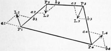
Fig. 86.

Considering, in the first place, the case in which the load and the two resistances by which each piece is balanced meet in one point, which may be called the centre of load, there will be as many such points of intersection, or centres of load, as there are pieces in the structure; and the directions and positions of the resistances or mutual pressures exerted between the pieces will be represented by the sides of a polygon joining those points, as in fig. 86 where P1, P2, P3, P4 represent the centres of load in a structure of four pieces, and the sides of the polygon of resistances P1 P2 P3 P4 represent respectively the directions and positions of the resistances exerted at the joints. Further, at any one of the centres of load let PL represent the magnitude and direction of the gross load, and Pa, Pb the two resistances by which the piece to which that load is applied is supported; then will those three lines be respectively the diagonal and sides of a parallelogram; or, what is the same thing, they will be equal to the three sides of a triangle; and they must be in the same plane, although the sides of the polygon of resistances may be in different planes.

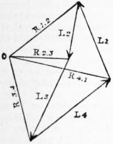
Fig. 87.

According to a well-known principle of statics, because the loads or external pressures P1L1, &c., balance each other, they must be proportional to the sides of a closed polygon drawn respectively parallel to their directions. In fig. 87 construct such a polygon of loads by drawing the lines L1, &c., parallel and proportional to, and joined end to end in the order of, the gross loads on the pieces of the structure. Then from the proportionality and parallelism of the load and the two resistances applied to each piece of the structure to the three sides of a triangle, there results the following theorem (originally due to Rankine):—

If from the angles of the polygon of loads there be drawn lines (R1, R2, &c.), each of which is parallel to the resistance (as P1P2, &c.) exerted at the joint between the pieces to which the two loads represented by the contiguous sides of the polygon of loads (such as L1, L2, &c.) are applied; then will all those lines meet in one point (O), and their lengths, measured from that point to the angles of the polygon, will represent the magnitudes of the resistances to which they are respectively parallel.

When the load on one of the pieces is parallel to the resistances which balance it, the polygon of resistances ceases to be closed, two of the sides becoming parallel to each other and to the load in question, and extending indefinitely. In the polygon of loads the direction of a load sustained by parallel resistances traverses the point O.2

§ 8. How the Earth’s Resistance is to be treated.... When the pressure exerted by a structure on the earth (to which the earth’s resistance is equal and opposite) consists either of one pressure, which is necessarily the resultant of the weight of the structure and of all the other forces applied to it, or of two or more parallel vertical forces, whose amount can be determined at the outset of the investigation, the resistance of the earth can be treated as one or more upward loads applied to the structure. But in other cases the earth is to be treated as one of the pieces of the structure, loaded with a force equal and opposite in direction and position to the resultant of the weight of the structure and of the other pressures applied to it.

§ 9. Partial Polygons of Resistance.—In a structure in which there are pieces supported at more than two joints, let a polygon be constructed of lines connecting the centres of load of any continuous series of pieces. This may be called a partial polygon of resistances. In considering its properties, the load at each centre of load is to be held to include the resistances of those joints which are not comprehended in the partial polygon of resistances, to which the theorem of § 7 will then apply in every respect. By constructing several partial polygons, and computing the relations between the loads and resistances which are determined by the application of that theorem to each of them, with the aid, if necessary, of Moseley’s principle of the least resistance, the whole of the relations amongst the loads and resistances may be found.

§ 10. Line of Pressures—Centres and Line of Resistance.—The line of pressures is a line to which the directions of all the resistances in one polygon are tangents. The centre of resistance at any joint is the point where the line representing the total resistance exerted at that joint intersects the joint. The line of resistance is a line traversing all the centres of resistance of a series of joints,—its form, in the positions intermediate between the actual joints of the structure, being determined by supposing the pieces and their loads to be subdivided by the introduction of intermediate joints ad infinitum, and finding the continuous line, curved or straight, in which the intermediate centres of resistance are all situated, however great their number. The difference between the line of resistance and the line of pressures was first pointed out by Moseley.

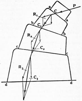
Fig. 88.

§ 11.* The principles of the two preceding sections may be illustrated by the consideration of a particular case of a buttress of blocks forming a continuous series of pieces (fig. 88), where aa, bb, cc, dd represent plane joints. Let the centre of pressure C at the first joint aa be known, and also the pressure P acting at C in direction and magnitude. Find R1 the resultant of this pressure, the weight of the block aabb acting through its centre of gravity, and any other external force which may be acting on the block, and produce its line of action to cut the joint bb in C1. C1 is then the centre of pressure for the joint bb, and R1 is the total force acting there. Repeating this process for each block in succession there will be found the centres of pressure C2, C3, &c., and also the resultant pressures R2, R3, &c., acting at these respective centres. The centres of pressure at the joints are also called centres of resistance, and the curve passing through these points is called a line of resistance. Let all the resultants acting at the several centres of resistance be produced until they cut one another in a series of points so as to form an unclosed polygon. This polygon is the partial polygon of resistance. A curve tangential to all the sides of the polygon is the line of pressures.

§ 12. Stability of Position, and Stability of Friction.—The resistances at the several joints having been determined by the principles set forth in §§ 6, 7, 8, 9 and 10, not only under the ordinary load of the structure, but under all the variations to which the load is subject as to amount and distribution, the joints are now to be placed and shaped so that the pieces shall not suffer relative displacement under any of those loads. The relative displacement of the two pieces which abut against each other at a joint may take place either by turning or by sliding. Safety against displacement by turning is called stability of position; safety against displacement by sliding, stability of friction.

§ 13. Condition of Stability of Position.—If the materials of a structure were infinitely stiff and strong, stability of position at any joint would be insured simply by making the centre of resistance fall within the joint under all possible variations of load. In order to allow for the finite stiffness and strength of materials, the least distance of the centre of resistance inward from the nearest edge of the joint is made to bear a definite proportion to the depth of the joint measured in the same direction, which proportion is fixed, sometimes empirically, sometimes by theoretical deduction from the laws of the strength of materials. That least distance is called by Moseley the modulus of stability. The following are some of the ratios of the modulus of stability to the depth of the joint which occur in practice:—

Retaining walls, as designed by British engineers 1 : 8

Retaining walls, as designed by French engineers 1 : 5

Rectangular piers of bridges and other buildings, and arch-stones 1 : 3

Rectangular foundations, firm ground 1 : 3

Rectangular foundations, very soft ground 1 : 2

Rectangular foundations, intermediate kinds of ground 1 : 3 to 1 : 2

Thin, hollow towers (such as furnace chimneys exposed to high winds), square 1 : 6

Thin, hollow towers, circular 1 : 4

Frames of timber or metal, under their ordinary or average distribution of load 1 : 3

Frames of timber or metal, under the greatest irregularities of load 1 : 3

In the case of the towers, the depth of the joint is to be understood to mean the diameter of the tower.

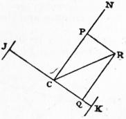
Fig. 89.

§ 14. Condition of Stability of Friction.—If the resistance to be exerted at a joint is always perpendicular to the surfaces which abut at and form that joint, there is no tendency of the pieces to be displaced by sliding. If the resistance be oblique, let JK (fig. 89) be the joint, C its centre of resistance, CR a line representing the resistance, CN a perpendicular to the joint at the centre of resistance. The angle NCR is the obliquity of the resistance. From R draw RP parallel and RQ perpendicular to the joint; then, by the principles of statics, the component of the resistance normal to the joint is—

CP = CR · cos PCR;

and the component tangential to the joint is—

CQ = CR · sin PCR = CP · tan PCR.

If the joint be provided either with projections and recesses, such as mortises and tenons, or with fastenings, such as pins or bolts, so as to resist displacement by sliding, the question of the utmost amount of the tangential resistance CQ which it is capable of exerting depends on the strength of such projections, recesses, or fastenings; and belongs to the subject of strength, and not to that of stability. In other cases the safety of the joint against displacement by sliding depends on its power of exerting friction, and that power depends on the law, known by experiment, that the friction between two surfaces bears a constant ratio, depending on the nature of the surfaces, to the force by which they are pressed together. In order that the surfaces which abut at the joint JK may be pressed together, the resistance required by the conditions of equilibrium CR, must be a thrust and not a pull; and in that case the force by which the surfaces are pressed together is equal and opposite to the normal component CP of the resistance. The condition of stability of friction is that the tangential component CQ of the resistance required shall not exceed the friction due to the normal component; that is, that

CQ ≯ ƒ · CP,

where ƒ denotes the coefficient of friction for the surfaces in question. The angle whose tangent is the coefficient of friction is called the angle of repose, and is expressed symbolically by—

φ = tan −1 ƒ.

Now CQ = CP · tan PCR;

consequently the condition of stability of friction is fulfilled if the angle PCR is not greater than φ; that is to say, if the obliquity of the resistance required at the joint does not exceed the angle of repose; and this condition ought to be fulfilled under all possible variations of the load.

It is chiefly in masonry and earthwork that stability of friction is relied on.

§ 15. Stability of Friction in Earth.—The grains of a mass of loose earth are to be regarded as so many separate pieces abutting against each other at joints in all possible positions, and depending for their stability on friction. To determine whether a mass of earth is stable at a given point, conceive that point to be traversed by planes in all possible positions, and determine which position gives the greatest obliquity to the total pressure exerted between the portions of the mass which abut against each other at the plane. The condition of stability is that this obliquity shall not exceed the angle of repose of the earth. The consequences of this principle are developed in a paper, “On the Stability of Loose Earth,” already cited in § 2.

§ 16. Parallel Projections of Figures.—If any figure be referred to a system of co-ordinates, rectangular or oblique, and if a second figure be constructed by means of a second system of co-ordinates, rectangular or oblique, and either agreeing with or differing from the first system in rectangularity or obliquity, but so related to the co-ordinates of the first figure that for each point in the first figure there shall be a corresponding point in the second figure, the lengths of whose co-ordinates shall bear respectively to the three corresponding co-ordinates of the corresponding point in the first figure three ratios which are the same for every pair of corresponding points in the two figures, these corresponding figures are called parallel projections of each other. The properties of parallel projections of most importance to the subject of the present article are the following:—

(1) A parallel projection of a straight line is a straight line.

(2) A parallel projection of a plane is a plane.

(3) A parallel projection of a straight line or a plane surface divided in a given ratio is a straight line or a plane surface divided in the same ratio.

(4) A parallel projection of a pair of equal and parallel straight lines, or plain surfaces, is a pair of equal and parallel straight lines, or plane surfaces; whence it follows

(5) That a parallel projection of a parallelogram is a parallelogram, and

(6) That a parallel projection of a parallelepiped is a parallelepiped.

(7) A parallel projection of a pair of solids having a given ratio is a pair of solids having the same ratio.

Though not essential for the purposes of the present article, the following consequence will serve to illustrate the principle of parallel projections:—

(8) A parallel projection of a curve, or of a surface of a given algebraical order, is a curve or a surface of the same order.

For example, all ellipsoids referred to co-ordinates parallel to any three conjugate diameters are parallel projections of each other and of a sphere referred to rectangular co-ordinates.

§ 17. Parallel Projections of Systems of Forces.—If a balanced system of forces be represented by a system of lines, then will every parallel projection of that system of lines represent a balanced system of forces.

For the condition of equilibrium of forces not parallel is that they shall be represented in direction and magnitude by the sides and diagonals of certain parallelograms, and of parallel forces that they shall divide certain straight lines in certain ratios; and the parallel projection of a parallelogram is a parallelogram, and that of a straight line divided in a given ratio is a straight line divided in the same ratio.

The resultant of a parallel projection of any system of forces is the projection of their resultant; and the centre of gravity of a parallel projection of a solid is the projection of the centre of gravity of the first solid.

§ 18. Principle of the Transformation of Structures.—Here we have the following theorem: If a structure of a given figure have stability of position under a system of forces represented by a given system of lines, then will any structure whose figure is a parallel projection of that of the first structure have stability of position under a system of forces represented by the corresponding projection of the first system of lines.

For in the second structure the weights, external pressures, and resistances will balance each other as in the first structure; the weights of the pieces and all other parallel systems of forces will have the same ratios as in the first structure; and the several centres of resistance will divide the depths of the joints in the same proportions as in the first structure.

If the first structure have stability of friction, the second structure will have stability of friction also, so long as the effect of the projection is not to increase the obliquity of the resistance at any joint beyond the angle of repose.

The lines representing the forces in the second figure show their relative directions and magnitudes. To find their absolute directions and magnitudes, a vertical line is to be drawn in the first figure, of such a length as to represent the weight of a particular portion of the structure. Then will the projection of that line in the projected figure indicate the vertical direction, and represent the weight of the part of the second structure corresponding to the before-mentioned portion of the first structure.

The foregoing “principle of the transformation of structures” was first announced, though in a somewhat less comprehensive form, to the Royal Society on the 6th of March 1856. It is useful in practice, by enabling the engineer easily to deduce the conditions of equilibrium and stability of structures of complex and unsymmetrical figures from those of structures of simple and symmetrical figures. By its aid, for example, the whole of the properties of elliptical arches, whether square or skew, whether level or sloping in their span, are at once deduced by projection from those of symmetrical circular arches, and the properties of ellipsoidal and elliptic-conoidal domes from those of hemispherical and circular-conoidal domes; and the figures of arches fitted to resist the thrust of earth, which is less horizontally than vertically in a certain given ratio, can be deduced by a projection from those of arches fitted to resist the thrust of a liquid, which is of equal intensity, horizontally and vertically.

§ 19. Conditions of Stiffness and Strength.—After the arrangement of the pieces of a structure and the size and figure of their joints or surfaces of contact have been determined so as to fulfil the conditions of stability,—conditions which depend mainly on the position and direction of the resultant or total load on each piece, and the relative magnitude of the loads on the different pieces—the dimensions of each piece singly have to be adjusted so as to fulfil the conditions of stiffness and strength—conditions which depend not only on the absolute magnitude of the load on each piece, and of the resistances by which it is balanced, but also on the mode of distribution of the load over the piece, and of the resistances over the joints.

The effect of the pressures applied to a piece, consisting of the load and the supporting resistances, is to force the piece into a state of strain or disfigurement, which increases until the elasticity, or resistance to strain, of the material causes it to exert a stress, or effort to recover its figure, equal and opposite to the system of applied pressures. The condition of stiffness is that the strain or disfigurement shall not be greater than is consistent with the purposes of the structure; and the condition of strength is that the stress shall be within the limits of that which the material can bear with safety against breaking. The ratio in which the utmost stress before breaking exceeds the safe working stress is called the factor of safety, and is determined empirically. It varies from three to twelve for various materials and structures. (See Strength of Materials.)

PART II. THEORY OF MACHINES

§ 20. Parts of a Machine: Frame and Mechanism.—The parts of a machine may be distinguished into two principal divisions,—the frame, or fixed parts, and the mechanism, or moving parts. The frame is a structure which supports the pieces of the mechanism, and to a certain extent determines the nature of their motions.

The form and arrangement of the pieces of the frame depend upon the arrangement and the motions of the mechanism; the dimensions of the pieces of the frame required in order to give it stability and strength are determined from the pressures applied to it by means of the mechanism. It appears therefore that in general the mechanism is to be designed first and the frame afterwards, and that the designing of the frame is regulated by the principles of the stability of structures and of the strength and stiffness of materials,—care being taken to adapt the frame to the most severe load which can be thrown upon it at any period of the action of the mechanism.

Each independent piece of the mechanism also is a structure, and its dimensions are to be adapted, according to the principles of the strength and stiffness of materials, to the most severe load to which it can be subjected during the action of the machine.

§ 21. Definition and Division of the Theory of Machines.—From what has been said in the last section it appears that the department of the art of designing machines which has reference to the stability of the frame and to the stiffness and strength of the frame and mechanism is a branch of the art of construction. It is therefore to be separated from the theory of machines, properly speaking, which has reference to the action of machines considered as moving. In the action of a machine the following three things take place:—

Firstly, Some natural source of energy communicates motion and force to a piece or pieces of the mechanism, called the receiver of power or prime mover.

Secondly, The motion and force are transmitted from the prime mover through the train of mechanism to the working piece or pieces, and during that transmission the motion and force are modified in amount and direction, so as to be rendered suitable for the purpose to which they are to be applied.

Thirdly, The working piece or pieces by their motion, or by their motion and force combined, produce some useful effect.

Such are the phenomena of the action of a machine, arranged in the order of causation. But in studying or treating of the theory of machines, the order of simplicity is the best; and in this order the first branch of the subject is the modification of motion and force by the train of mechanism; the next is the effect or purpose of the machine; and the last, or most complex, is the action of the prime mover.

The modification of motion and the modification of force take place together, and are connected by certain laws; but in the study of the theory of machines, as well as in that of pure mechanics, much advantage has been gained in point of clearness and simplicity by first considering alone the principles of the modification of motion, which are founded upon what is now known as Kinematics, and afterwards considering the principles of the combined modification of motion and force, which are founded both on geometry and on the laws of dynamics. The separation of kinematics from dynamics is due mainly to G. Monge, Ampère and R. Willis.

The theory of machines in the present article will be considered under the following heads:—

I. Pure Mechanism, or Applied Kinematics; being the theory of machines considered simply as modifying motion.

II. Applied Dynamics; being the theory of machines considered as modifying both motion and force.

Chap. I. On Pure Mechanism

§ 22. Division of the Subject.—Proceeding in the order of simplicity, the subject of Pure Mechanism, or Applied Kinematics, may be thus divided:—

Division 1.—Motion of a point.

Division 2.—Motion of the surface of a fluid.

Division 3.—Motion of a rigid solid.

Division 4.—Motions of a pair of connected pieces, or of an “elementary combination” in mechanism.

Division 5.—Motions of trains of pieces of mechanism.

Division 6.—Motions of sets of more than two connected pieces, or of “aggregate combinations.”

A point is the boundary of a line, which is the boundary of a surface, which is the boundary of a volume. Points, lines and surfaces have no independent existence, and consequently those divisions of this chapter which relate to their motions are only preliminary to the subsequent divisions, which relate to the motions of bodies.

Division 1. Motion of a Point.

§ 23. Comparative Motion.—The comparative motion of two points is the relation which exists between their motions, without having regard to their absolute amounts. It consists of two elements,—the velocity ratio, which is the ratio of any two magnitudes bearing to each other the proportions of the respective velocities of the two points at a given instant, and the directional relation, which is the relation borne to each other by the respective directions of the motions of the two points at the same given instant.

It is obvious that the motions of a pair of points may be varied in any manner, whether by direct or by lateral deviation, and yet that their comparative motion may remain constant, in consequence of the deviations taking place in the same proportions, in the same directions and at the same instants for both points.

Robert Willis (1800-1875) has the merit of having been the first to simplify considerably the theory of pure mechanism, by pointing out that that branch of mechanics relates wholly to comparative motions.

The comparative motion of two points at a given instant is capable of being completely expressed by one of Sir William Hamilton’s Quaternions,—the “tensor” expressing the velocity ratio, and the “versor” the directional relation.

Graphical methods of analysis founded on this way of representing velocity and acceleration were developed by R. H. Smith in a paper communicated to the Royal Society of Edinburgh in 1885, and illustrations of the method will be found below.

Division 2. Motion of the Surface of a Fluid Mass.

§ 24. General Principle.—A mass of fluid is used in mechanism to transmit motion and force between two or more movable portions (called pistons or plungers) of the solid envelope or vessel in which the fluid is contained; and, when such transmission is the sole action, or the only appreciable action of the fluid mass, its volume is either absolutely constant, by reason of its temperature and pressure being maintained constant, or not sensibly varied.

Let a represent the area of the section of a piston made by a plane perpendicular to its direction of motion, and v its velocity, which is to be considered as positive when outward, and negative when inward. Then the variation of the cubic contents of the vessel in a unit of time by reason of the motion of one piston is va. The condition that the volume of the fluid mass shall remain unchanged requires that there shall be more than one piston, and that the velocities and areas of the pistons shall be connected by the equation—

Σ · va = 0.

(1)

§ 25. Comparative Motion of Two Pistons.—If there be but two pistons, whose areas are a1 and a2, and their velocities v1 and v2, their comparative motion is expressed by the equation—

v2/v1 = −a1/a2;

(2)

that is to say, their velocities are opposite as to inwardness and outwardness and inversely proportional to their areas.

§ 26. Applications: Hydraulic Press: Pneumatic Power-Transmitter.—In the hydraulic press the vessel consists of two cylinders, viz. the pump-barrel and the press-barrel, each having its piston, and of a passage connecting them having a valve opening towards the press-barrel. The action of the enclosed water in transmitting motion takes place during the inward stroke of the pump-plunger, when the above-mentioned valve is open; and at that time the press-plunger moves outwards with a velocity which is less than the inward velocity of the pump-plunger, in the same ratio that the area of the pump-plunger is less than the area of the press-plunger. (See Hydraulics.)

In the pneumatic power-transmitter the motion of one piston is transmitted to another at a distance by means of a mass of air contained in two cylinders and an intervening tube. When the pressure and temperature of the air can be maintained constant, this machine fulfils equation (2), like the hydraulic press. The amount and effect of the variations of pressure and temperature undergone by the air depend on the principles of the mechanical action of heat, or Thermodynamics (q.v.), and are foreign to the subject of pure mechanism.

Division 3. Motion of a Rigid Solid.

§ 27. Motions Classed.—In problems of mechanism, each solid piece of the machine is supposed to be so stiff and strong as not to undergo any sensible change of figure or dimensions by the forces applied to it—a supposition which is realized in practice if the machine is skilfully designed.

This being the case, the various possible motions of a rigid solid body may all be classed under the following heads: (1) Shifting or Translation; (2) Turning or Rotation; (3) Motions compounded of Shifting and Turning.

The most common forms for the paths of the points of a piece of mechanism, whose motion is simple shifting, are the straight line and the circle.

Shifting in a straight line is regulated either by straight fixed guides, in contact with which the moving piece slides, or by combinations of link-work, called parallel motions, which will be described in the sequel. Shifting in a straight line is usually reciprocating; that is to say, the piece, after shifting through a certain distance, returns to its original position by reversing its motion.

Circular shifting is regulated by attaching two or more points of the shifting piece to ends of equal and parallel rotating cranks, or by combinations of wheel-work to be afterwards described. As an example of circular shifting may be cited the motion of the coupling rod, by which the parallel and equal cranks upon two or more axles of a locomotive engine are connected and made to rotate simultaneously. The coupling rod remains always parallel to itself, and all its points describe equal and similar circles relatively to the frame of the engine, and move in parallel directions with equal velocities at the same instant.

§ 28. Rotation about a Fixed Axis: Lever, Wheel and Axle.—The fixed axis of a turning body is a line fixed relatively to the body and relatively to the fixed space in which the body turns. In mechanism it is usually the central line either of a rotating shaft or axle having journals, gudgeons, or pivots turning in fixed bearings, or of a fixed spindle or dead centre round which a rotating bush turns; but it may sometimes be entirely beyond the limits of the turning body. For example, if a sliding piece moves in circular fixed guides, that piece rotates about an ideal fixed axis traversing the centre of those guides.

Let the angular velocity of the rotation be denoted by α = dθ/dt, then the linear velocity of any point A at the distance r from the axis is αr; and the path of that point is a circle of the radius r described about the axis.

This is the principle of the modification of motion by the lever, which consists of a rigid body turning about a fixed axis called a fulcrum, and having two points at the same or different distances from that axis, and in the same or different directions, one of which receives motion and the other transmits motion, modified in direction and velocity according to the above law.

In the wheel and axle, motion is received and transmitted by two cylindrical surfaces of different radii described about their common fixed axis of turning, their velocity-ratio being that of their radii.

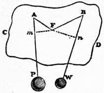
Fig. 90.

§ 29. Velocity Ratio of Components of Motion.—As the distance between any two points in a rigid body is invariable, the projections of their velocities upon the line joining them must be equal. Hence it follows that, if A in fig. 90 be a point in a rigid body CD, rotating round the fixed axis F, the component of the velocity of A in any direction AP parallel to the plane of rotation is equal to the total velocity of the point m, found by letting fall Fm perpendicular to AP; that is to say, is equal to

α · Fm.

Hence also the ratio of the components of the velocities of two points A and B in the directions AP and BW respectively, both in the plane of rotation, is equal to the ratio of the perpendiculars Fm and Fn.

§ 30. Instantaneous Axis of a Cylinder rolling on a Cylinder.—Let a cylinder bbb, whose axis of figure is B and angular velocity γ, roll on a fixed cylinder ααα, whose axis of figure is A, either outside (as in fig. 91), when the rolling will be towards the same hand as the rotation, or inside (as in fig. 92), when the rolling will be towards the opposite hand; and at a given instant let T be the line of contact of the two cylindrical surfaces, which is at their common intersection with the plane AB traversing the two axes of figure.

The line T on the surface bbb has for the instant no velocity in a direction perpendicular to AB; because for the instant it touches, without sliding, the line T on the fixed surface aaa.

The line T on the surface bbb has also for the instant no velocity in the plane AB; for it has just ceased to move towards the fixed surface aaa, and is just about to begin to move away from that surface.

The line of contact T, therefore, on the surface of the cylinder bbb, is for the instant at rest, and is the “instantaneous axis” about which the cylinder bbb turns, together with any body rigidly attached to that cylinder.

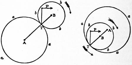
Fig. 91. Fig. 92.

To find, then, the direction and velocity at the given instant of any point P, either in or rigidly attached to the rolling cylinder T, draw the plane PT; the direction of motion of P will be perpendicular to that plane, and towards the right or left hand according to the direction of the rotation of bbb; and the velocity of P will be

vP = γ·PT,

(3)

PT denoting the perpendicular distance of P from T. The path of P is a curve of the kind called epitrochoids. If P is in the circumference of bbb, that path becomes an epicycloid.

The velocity of any point in the axis of figure B is

vB = γ·TB;

(4)

and the path of such a point is a circle described about A with the radius AB, being for outside rolling the sum, and for inside rolling the difference, of the radii of the cylinders.

Let α denote the angular velocity with which the plane of axes AB rotates about the fixed axis A. Then it is evident that

vB = α·AB,

(5)

and consequently that

α = γ·TB/AB.

(6)

For internal rolling, as in fig. 92, AB is to be treated as negative, which will give a negative value to α, indicating that in this case the rotation of AB round A is contrary to that of the cylinder bbb.

The angular velocity of the rolling cylinder, relatively to the plane of axes AB, is obviously given by the equation—

β = γ − α

whence β = γ · TA/AB

(7)

care being taken to attend to the sign of α, so that when that is negative the arithmetical values of γ and α are to be added in order to give that of β.

The whole of the foregoing reasonings are applicable, not merely when aaa and bbb are actual cylinders, but also when they are the osculating cylinders of a pair of cylindroidal surfaces of varying curvature, A and B being the axes of curvature of the parts of those surfaces which are in contact for the instant under consideration.

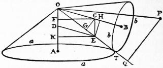
Fig. 93.

§ 31. Instantaneous Axis of a Cone rolling on a Cone.—Let Oaa (fig. 93) be a fixed cone, OA its axis, Obb a cone rolling on it, OB the axis of the rolling cone, OT the line of contact of the two cones at the instant under consideration. By reasoning similar to that of § 30, it appears that OT is the instantaneous axis of rotation of the rolling cone.

Let γ denote the total angular velocity of the rotation of the cone B about the instantaneous axis, β its angular velocity about the axis OB relatively to the plane AOB, and α the angular velocity with which the plane AOB turns round the axis OA. It is required to find the ratios of those angular velocities.

Solution.—In OT take any point E, from which draw EC parallel to OA, and ED parallel to OB, so as to construct the parallelogram OCED. Then

OD : OC : OE :: α : β : γ.

(8)

Or because of the proportionality of the sides of triangles to the sines of the opposite angles,

sin TOB : sin TOA : sin AOB :: α : β : γ,

(8 A)

that is to say, the angular velocity about each axis is proportional to the sine of the angle between the other two.

Demonstration.—From C draw CF perpendicular to OA, and CG perpendicular to OE

Then CF = 2 × area EC ,

CE

and CG = 2 × area ECO ;

OE

∴ CG : CF :: CE = OD : OE.

Let vc denote the linear velocity of the point C. Then

vc = α · CF = γ · CG ∴ γ : α :: CF : CG :: OE : OD,

which is one part of the solution above stated. From E draw EH perpendicular to OB, and EK to OA. Then it can be shown as before that

EK : EH :: OC : OD.

Let vE be the linear velocity of the point E fixed in the plane of axes AOB. Then

vK = α · EK.

Now, as the line of contact OT is for the instant at rest on the rolling cone as well as on the fixed cone, the linear velocity of the point E fixed to the plane AOB relatively to the rolling cone is the same with its velocity relatively to the fixed cone. That is to say,

β · EH = vE = α · EK;

therefore

α : β :: EH : EK :: OD : OC,

which is the remainder of the solution.

The path of a point P in or attached to the rolling cone is a spherical epitrochoid traced on the surface of a sphere of the radius OP. From P draw PQ perpendicular to the instantaneous axis. Then the motion of P is perpendicular to the plane OPQ, and its velocity is

vP = γ · PQ.

(9)

The whole of the foregoing reasonings are applicable, not merely when A and B are actual regular cones, but also when they are the osculating regular cones of a pair of irregular conical surfaces, having a common apex at O.

§ 32. Screw-like or Helical Motion.—Since any displacement in a plane can be represented in general by a rotation, it follows that the only combination of translation and rotation, in which a complex movement which is not a mere rotation is produced, occurs when there is a translation perpendicular to the plane and parallel to the axis of rotation.

Fig. 94.

Such a complex motion is called screw-like or helical motion; for each point in the body describes a helix or screw round the axis of rotation, fixed or instantaneous as the case may be. To cause a body to move in this manner it is usually made of a helical or screw-like figure, and moves in a guide of a corresponding figure. Helical motion and screws adapted to it are said to be right- or left-handed according to the appearance presented by the rotation to an observer looking towards the direction of the translation. Thus the screw G in fig. 94 is right-handed.

The translation of a body in helical motion is called its advance. Let vx denote the velocity of advance at a given instant, which of course is common to all the particles of the body; α the angular velocity of the rotation at the same instant; 2π = 6.2832 nearly, the circumference of a circle of the radius unity. Then

T = 2π/α

(10)

is the time of one turn at the rate α; and

p = vxT = 2πvx/α

(11)

is the pitch or advance per turn—a length which expresses the comparative motion of the translation and the rotation.

The pitch of a screw is the distance, measured parallel to its axis, between two successive turns of the same thread or helical projection.

Let r denote the perpendicular distance of a point in a body moving helically from the axis. Then

vr = αr

(12)

is the component of the velocity of that point in a plane perpendicular to the axis, and its total velocity is

v = √ {vx2 + vr2}.

(13)

The ratio of the two components of that velocity is

vx/vr = p/2πr = tan θ.

(14)

where θ denotes the angle made by the helical path of the point with a plane perpendicular to the axis.

Division 4. Elementary Combinations in Mechanism

§ 33. Definitions.—An elementary combination in mechanism consists of two pieces whose kinds of motion are determined by their connexion with the frame, and their comparative motion by their connexion with each other—that connexion being effected either by direct contact of the pieces, or by a connecting piece, which is not connected with the frame, and whose motion depends entirely on the motions of the pieces which it connects.

The piece whose motion is the cause is called the driver; the piece whose motion is the effect, the follower.

The connexion of each of those two pieces with the frame is in general such as to determine the path of every point in it. In the investigation, therefore, of the comparative motion of the driver and follower, in an elementary combination, it is unnecessary to consider relations of angular direction, which are already fixed by the connexion of each piece with the frame; so that the inquiry is confined to the determination of the velocity ratio, and of the directional relation, so far only as it expresses the connexion between forward and backward movements of the driver and follower. When a continuous motion of the driver produces a continuous motion of the follower, forward or backward, and a reciprocating motion a motion reciprocating at the same instant, the directional relation is said to be constant. When a continuous motion produces a reciprocating motion, or vice versa, or when a reciprocating motion produces a motion not reciprocating at the same instant, the directional relation is said to be variable.

The line of action or of connexion of the driver and follower is a line traversing a pair of points in the driver and follower respectively, which are so connected that the component of their velocity relatively to each other, resolved along the line of connexion, is null. There may be several or an indefinite number of lines of connexion, or there may be but one; and a line of connexion may connect either the same pair of points or a succession of different pairs.