VOLUME XVII SLICE VIII Matter to Mecklenburg (continued 8)

L1 = y1Z1 − z1Y1, M1 = z1X1 − x1Z1, N1 = x1Y1 − y1X1.

(5)

It is seen that L1, M1, N1 are the moments of the original force at P1 about the co-ordinate axes. Summing up for all the forces of the given system, we obtain a force R at O, whose components are

X = Σ(Xr), Y = Σ(Yr), Z = Σ(Zr),

(6)

and a couple G whose components are

L = Σ(Lr), M = Σ(Mr), N = Σ(Nr),

(7)

where r = 1, 2, 3 ... Since R2 = X2 + Y2 + Z2, G2 = L2 + M2 + N2, it is necessary and sufficient for equilibrium that the six quantities X, Y, Z, L, M, N, should all vanish. In words: the sum of the projections of the forces on each of the co-ordinate axes must vanish; and, the sum of the moments of the forces about each of these axes must vanish.

If any other point O′, whose co-ordinates are x, y, z, be chosen in place of O, as the point to which the forces are transferred, we have to write x1 − x, y1 − y, z1 − z for x1, y1, z1, and so on, in the preceding process. The components of the resultant force R are unaltered, but the new components of couple are found to be

L′ = L − yZ + zY, M′ = M − zX + xZ, N′ = N − xY + yX.

(8)

By properly choosing O′ we can make the plane of the couple perpendicular to the resultant force. The conditions for this are L′ : M′ : N′ = X : Y : Z, or

L − yZ + zY = M − zX + xZ = N − xY + yX

X Y Z

(9)

These are the equations of the central axis. Since the moment of the resultant couple is now

G′ = X L′ + Y M′ + Z N′ = LX + MY + NZ ,

R R R R

(10)

the pitch of the equivalent wrench is

(LX + MY + NZ) / (X2 + Y2 + Z2).

It appears that X2 + Y2 + Z2 and LX + MY + NZ are absolute invariants (cf. § 7). When the latter invariant, but not the former, vanishes, the system reduces to a single force.

The analogy between the mathematical relations of infinitely small displacements on the one hand and those of force-systems on the other enables us immediately to convert any theorem in the one subject into a theorem in the other. For example, we can assert without further proof that any infinitely small displacement may be resolved into two rotations, and that the axis of one of these can be chosen arbitrarily. Again, that wrenches of arbitrary amounts about two given screws compound into a wrench the locus of whose axis is a cylindroid.

The mathematical properties of a twist or of a wrench have been the subject of many remarkable investigations, which are, however, of secondary importance from a physical point of view. In the “Null-System” of A. F. Möbius (1790-1868), a line such that the moment of a given wrench about it is zero is called a null-line. The triply infinite system of null-lines form what is called in line-geometry a “complex.” As regards the configuration of this complex, consider a line whose shortest distance from the central axis is r, and whose inclination to the central axis is θ. The moment of the resultant force R of the wrench about this line is − Rr sin θ, and that of the couple G is G cos θ. Hence the line will be a null-line provided

tan θ = k/r,

(11)

where k is the pitch of the wrench. The null-lines which are at a given distance r from a point O of the central axis will therefore form one system of generators of a hyperboloid of revolution; and by varying r we get a series of such hyperboloids with a common centre and axis. By moving O along the central axis we obtain the whole complex of null-lines. It appears also from (11) that the null-lines whose distance from the central axis is r are tangent lines to a system of helices of slope tan−1 (r/k); and it is to be noticed that these helices are left-handed if the given wrench is right-handed, and vice versa.

Since the given wrench can be replaced by a force acting through any assigned point P, and a couple, the locus of the null-lines through P is a plane, viz. a plane perpendicular to the vector which represents the couple. The complex is therefore of the type called “linear” (in relation to the degree of this locus). The plane in question is called the null-plane of P. If the null-plane of P pass through Q, the null-plane of Q will pass through P, since PQ is a null-line. Again, any plane ω is the locus of a system of null-lines meeting in a point, called the null-point of ω. If a plane revolve about a fixed straight line p in it, its null-point describes another straight line p′, which is called the conjugate line of p. We have seen that the wrench may be replaced by two forces, one of which may act in any arbitrary line p. It is now evident that the second force must act in the conjugate line p′, since every line meeting p, p′ is a null-line. Again, since the shortest distance between any two conjugate lines cuts the central axis at right angles, the orthogonal projections of two conjugate lines on a plane perpendicular to the central axis will be parallel (fig. 42). This property was employed by L. Cremona to prove the existence under certain conditions of “reciprocal figures” in a plane (§ 5). If we take any polyhedron with plane faces, the null-planes of its vertices with respect to a given wrench will form another polyhedron, and the edges of the latter will be conjugate (in the above sense) to those of the former. Projecting orthogonally on a plane perpendicular to the central axis we obtain two reciprocal figures.

In the analogous theory of infinitely small displacements of a solid, a “null-line” is a line such that the lengthwise displacement of any point on it is zero.

Since a wrench is defined by six independent quantities, it can in general be replaced by any system of forces which involves six adjustable elements. For instance, it can in general be replaced by six forces acting in six given lines, e.g. in the six edges of a given tetrahedron. An exception to the general statement occurs when the six lines are such that they are possible lines of action of a system of six forces in equilibrium; they are then said to be in involution. The theory of forces in involution has been studied by A. Cayley, J. J. Sylvester and others. We have seen that a rigid structure may in general be rigidly connected with the earth by six links, and it now appears that any system of forces acting on the structure can in general be balanced by six determinate forces exerted by the links. If, however, the links are in involution, these forces become infinite or indeterminate. There is a corresponding kinematic peculiarity, in that the connexion is now not strictly rigid, an infinitely small relative displacement being possible. See § 9.

When parallel forces of given magnitudes act at given points, the resultant acts through a definite point, or centre of parallel forces, which is independent of the special direction of the forces. If Pr be the force at (xr, yr, zr), acting in the direction (l, m, n), the formulae (6) and (7) reduce to

X = Σ(P)·l, Y = Σ(P)·m, Z = Σ(P)·n,

(12)

and

L = Σ(P)·(ny − mz), M = Σ(P)·(lz − nx), N = Σ(P)·(mx − ly),

(13)

provided

x = Σ(Px) , y = Σ(Py) , z = Σ(Pz) .

Σ(P) Σ(P) Σ(P)

(14)

These are the same as if we had a single force Σ(P) acting at the point (x, y, z), which is the same for all directions (l, m, n). We can hence derive the theory of the centre of gravity, as in § 4. An exceptional case occurs when Σ(P) = 0.

If we imagine a rigid body to be acted on at given points by forces of given magnitudes in directions (not all parallel) which are fixed in space, then as the body is turned about the resultant wrench will assume different configurations in the body, and will in certain positions reduce to a single force. The investigation of such questions forms the subject of “Astatics,” which has been cultivated by Möbius, Minding, G. Darboux and others. As it has no physical bearing it is passed over here.

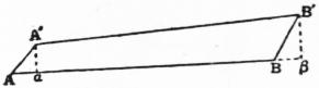
Fig. 45.

§ 9. Work.—The work done by a force acting on a particle, in any infinitely small displacement, is defined as the product of the force into the orthogonal projection of the displacement on the direction of the force; i.e. it is equal to F·δs cos θ, where F is the force, δs the displacement, and θ is the angle between the directions of F and δs. In the language of vector analysis (q.v.) it is the “scalar product” of the vector representing the force and the displacement. In the same way, the work done by a force acting on a rigid body in any infinitely small displacement of the body is the scalar product of the force into the displacement of any point on the line of action. This product is the same whatever point on the line of action be taken, since the lengthwise components of the displacements of any two points A, B on a line AB are equal, to the first order of small quantities. To see this, let A′, B′ be the displaced positions of A, B, and let φ be the infinitely small angle between AB and A′B′. Then if α, β be the orthogonal projections of A′, B′ on AB, we have

Aα − Bβ = AB − αβ = AB (1 − cos φ) = 1⁄2AB·φ2,

ultimately. Since this is of the second order, the products F·Aα and F·Bβ are ultimately equal.

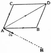
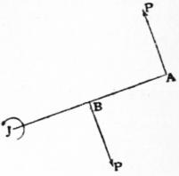
Fig. 46. Fig. 47.

The total work done by two concurrent forces acting on a particle, or on a rigid body, in any infinitely small displacement, is equal to the work of their resultant. Let AB, AC (fig. 46) represent the forces, AD their resultant, and let AH be the direction of the displacement δs of the point A. The proposition follows at once from the fact that the sum of orthogonal projections of AB>, AC> on AH is equal to the projection of AD>. It is to be noticed that AH need not be in the same plane with AB, AC.

It follows from the preceding statements that any two systems of forces which are statically equivalent, according to the principles of §§ 4, 8, will (to the first order of small quantities) do the same amount of work in any infinitely small displacement of a rigid body to which they may be applied. It is also evident that the total work done in two or more successive infinitely small displacements is equal to the work done in the resultant displacement.

The work of a couple in any infinitely small rotation of a rigid body about an axis perpendicular to the plane of the couple is equal to the product of the moment of the couple into the angle of rotation, proper conventions as to sign being observed. Let the couple consist of two forces P, P (fig. 47) in the plane of the paper, and let J be the point where this plane is met by the axis of rotation. Draw JBA perpendicular to the lines of action, and let ε be the angle of rotation. The work of the couple is

P·JA·ε − P·JB·ε = P·AB·ε = Gε,

if G be the moment of the couple.

The analytical calculation of the work done by a system of forces in any infinitesimal displacement is as follows. For a two-dimensional system we have, in the notation of §§ 3, 4,

Σ(Xδx + Yδy) = Σ{X(λ − yε) + Y(μ + xε)}

= Σ(X)·λ + Σ(Y)·μ + Σ(xY − yX) ε

= Xλ + Yμ + Nε.

(1)

Again, for a three-dimensional system, in the notation of §§ 7, 8,

Σ(Xδx + Yδy + Zδz)

= Σ{(X(λ + ηz − ζy) + Y(μ + ζx − ξx) + Z(ν + ξy − ηx)}

= Σ(X)·λ + Σ(Y)·μ + Σ(Z)·ν + Σ(yZ − zY)·ξ + Σ(zX − xZ)·η + Σ(xY − yX)·ζ

= Xλ + Yμ + Zν + Lξ + Mη + Nζ.

(2)

This expression gives the work done by a given wrench when the body receives a given infinitely small twist; it must of course be an absolute invariant for all transformations of rectangular axes. The first three terms express the work done by the components of a force (X, Y, Z) acting at O, and the remaining three terms express the work of a couple (L, M, N).

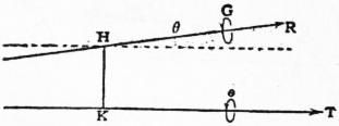
Fig. 48.

The work done by a wrench about a given screw, when the body twists about a second given screw, may be calculated directly as follows. In fig. 48 let R, G be the force and couple of the wrench, ε,τ the rotation and translation in the twist. Let the axes of the wrench and the twist be inclined at an angle θ, and let h be the shortest distance between them. The displacement of the point H in the figure, resolved in the direction of R, is τ cos θ − εh sin θ. The work is therefore

R (τ cos θ − εh sin θ) + G cos θ = Rε {(p + p′) cos θ − h sin θ},

(3)

if G = pR, τ = p′ε, i.e. p, p′ are the pitches of the two screws. The factor (p + p′) cos θ − h sin θ is called the virtual coefficient of the two screws which define the types of the wrench and twist, respectively.

A screw is determined by its axis and its pitch, and therefore involves five Independent elements. These may be, for instance, the five ratios ξ : η : ζ : λ : μ : ν of the six quantities which specify an infinitesimal twist about the screw. If the twist is a pure rotation, these quantities are subject to the relation

λξ + μη + νζ = 0.

(4)

In the analytical investigations of line geometry, these six quantities, supposed subject to the relation (4), are used to specify a line, and are called the six “co-ordinates” of the line; they are of course equivalent to only four independent quantities. If a line is a null-line with respect to the wrench (X, Y, Z, L, M, N), the work done in an infinitely small rotation about it is zero, and its co-ordinates are accordingly subject to the further relation

Lξ + Mη + Nζ + Xλ + Yμ + Zν = 0,

(5)

where the coefficients are constant. This is the equation of a “linear complex” (cf. § 8).

Two screws are reciprocal when a wrench about one does no work on a body which twists about the other. The condition for this is

λξ′ + μη′ + νζ′ + λ′ξ + μ′η + ν′ζ = 0,

(6)

if the screws be defined by the ratios ξ : η : ζ : λ : μ : ν and ξ′ : η′ : ζ′ : λ′ : μ′ : ν′, respectively. The theory of the screw-systems which are reciprocal to one, two, three, four given screws respectively has been investigated by Sir R. S. Ball.

Considering a rigid body in any given position, we may contemplate the whole group of infinitesimal displacements which might be given to it. If the extraneous forces are in equilibrium the total work which they would perform in any such displacement would be zero, since they reduce to a zero force and a zero couple. This is (in part) the celebrated principle of virtual velocities, now often described as the principle of virtual work, enunciated by John Bernoulli (1667-1748). The word “virtual” is used because the displacements in question are not regarded as actually taking place, the body being in fact at rest. The “velocities” referred to are the velocities of the various points of the body in any imagined motion of the body through the position in question; they obviously bear to one another the same ratios as the corresponding infinitesimal displacements. Conversely, we can show that if the virtual work of the extraneous forces be zero for every infinitesimal displacement of the body as rigid, these forces must be in equilibrium. For by giving the body (in imagination) a displacement of translation we learn that the sum of the resolved parts of the forces in any assigned direction is zero, and by giving it a displacement of pure rotation we learn that the sum of the moments about any assigned axis is zero. The same thing follows of course from the analytical expression (2) for the virtual work. If this vanishes for all values of λ, μ, ν, ξ, η, ζ we must have X, Y, Z, L, M, N = 0, which are the conditions of equilibrium.

The principle can of course be extended to any system of particles or rigid bodies, connected together in any way, provided we take into account the internal stresses, or reactions, between the various parts. Each such reaction consists of two equal and opposite forces, both of which may contribute to the equation of virtual work.

The proper significance of the principle of virtual work, and of its converse, will appear more clearly when we come to kinetics (§ 16); for the present it may be regarded merely as a compact and (for many purposes) highly convenient summary of the laws of equilibrium. Its special value lies in this, that by a suitable adjustment of the hypothetical displacements we are often enabled to eliminate unknown reactions. For example, in the case of a particle lying on a smooth curve, or on a smooth surface, if it be displaced along the curve, or on the surface, the virtual work of the normal component of the pressure may be ignored, since it is of the second order. Again, if two bodies are connected by a string or rod, and if the hypothetical displacements be adjusted so that the distance between the points of attachment is unaltered, the corresponding stress may be ignored. This is evident from fig. 45; if AB, A′B′ represent the two positions of a string, and T be the tension, the virtual work of the two forces ±T at A, B is T(Aα − Bβ), which was shown to be of the second order. Again, the normal pressure between two surfaces disappears from the equation, provided the displacements be such that one of these surfaces merely slides relatively to the other. It is evident, in the first place, that in any displacement common to the two surfaces, the work of the two equal and opposite normal pressures will cancel; moreover if, one of the surfaces being fixed, an infinitely small displacement shifts the point of contact from A to B, and if A′ be the new position of that point of the sliding body which was at A, the projection of AA′ on the normal at A is of the second order. It is to be noticed, in this case, that the tangential reaction (if any) between the two surfaces is not eliminated. Again, if the displacements be such that one curved surface rolls without sliding on another, the reaction, whether normal or tangential, at the point of contact may be ignored. For the virtual work of two equal and opposite forces will cancel in any displacement which is common to the two surfaces; whilst, if one surface be fixed, the displacement of that point of the rolling surface which was in contact with the other is of the second order. We are thus able to imagine a great variety of mechanical systems to which the principle of virtual work can be applied without any regard to the internal stresses, provided the hypothetical displacements be such that none of the connexions of the system are violated.

If the system be subject to gravity, the corresponding part of the virtual work can be calculated from the displacement of the centre of gravity. If W1, W2, ... be the weights of a system of particles, whose depths below a fixed horizontal plane of reference are z1, z2, ..., respectively, the virtual work of gravity is

W1δ·z1 + W2δz2 + ... = δ(W1z1 + W2z2 + ...) = (W1 + W2 + ...) δz,

where z is the depth of the centre of gravity (see § 8 (14) and § 11 (6)). This expression is the same as if the whole mass were concentrated at the centre of gravity, and displaced with this point. An important conclusion is that in any displacement of a system of bodies in equilibrium, such that the virtual work of all forces except gravity may be ignored, the depth of the centre of gravity is “stationary.”

The question as to stability of equilibrium belongs essentially to kinetics; but we may state by anticipation that in cases where gravity is the only force which does work, the equilibrium of a body or system of bodies is stable only if the depth of the centre of gravity be a maximum.

Consider, for instance, the case of a bar resting with its ends on two smooth inclines (fig. 18). If the bar be displaced in a vertical plane so that its ends slide on the two inclines, the instantaneous centre is at the point J. The displacement of G is at right angles to JG; this shows that for equilibrium JG must be vertical. Again, the locus of G is an arc of an ellipse whose centre is in the intersection of the planes; since this arc is convex upwards the equilibrium is unstable. A general criterion for the case of a rigid body movable in two dimensions, with one degree of freedom, can be obtained as follows. We have seen (§ 3) that the sequence of possible positions is obtained if we imagine the “body-centrode” to roll on the “space-centrode.” For equilibrium, the altitude of the centre of gravity G must be stationary; hence G must lie in the same vertical line with the point of contact J of the two curves. Further, it is known from the theory of “roulettes” that the locus of G will be concave or convex upwards according as

cos φ = 1 + 1 ,

h ρ ρ′

(8)

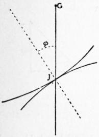
Fig. 49.

where ρ, ρ′ are the radii of curvature of the two curves at J, φ is the inclination of the common tangent at J to the horizontal, and h is the height of G above J. The signs of ρ, ρ′ are to be taken positive when the curvatures are as in the standard case shown in fig. 49. Hence for stability the upper sign must obtain in (8). The same criterion may be arrived at in a more intuitive manner as follows. If the body be supposed to roll (say to the right) until the curves touch at J′, and if JJ′ = δs, the angle through which the upper figure rotates is δs/ρ + δs/ρ′, and the horizontal displacement of G is equal to the product of this expression into h. If this displacement be less than the horizontal projection of JJ′, viz. δs cosφ, the vertical through the new position of G will fall to the left of J′ and gravity will tend to restore the body to its former position. It is here assumed that the remaining forces acting on the body in its displaced position have zero moment about J′; this is evidently the case, for instance, in the problem of “rocking stones.”

The principle of virtual work is specially convenient in the theory of frames (§ 6), since the reactions at smooth joints and the stresses in inextensible bars may be left out of account. In particular, in the case of a frame which is just rigid, the principle enables us to find the stress in any one bar independently of the rest. If we imagine the bar in question to be removed, equilibrium will still persist if we introduce two equal and opposite forces S, of suitable magnitude, at the joints which it connected. In any infinitely small deformation of the frame as thus modified, the virtual work of the forces S, together with that of the original extraneous forces, must vanish; this determines S.

As a simple example, take the case of a light frame, whose bars form the slides of a rhombus ABCD with the diagonal BD, suspended from A and carrying a weight W at C; and let it be required to find the stress in BD. If we remove the bar BD, and apply two equal and opposite forces S at B and D, the equation is

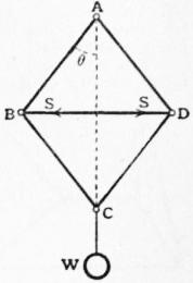
Fig. 50.

W·δ(2l cosθ) + 2S·δ (l sin θ) = 0,

where l is the length of a side of the rhombus, and θ its inclination to the vertical. Hence

S = W tan θ = W · BD/AC.

(8)

The method is specially appropriate when the frame, although just rigid, is not “simple” in the sense of § 6, and when accordingly the method of reciprocal figures is not immediately available. To avoid the intricate trigonometrical calculations which would often be necessary, graphical devices have been introduced by H. Müller-Breslau and others. For this purpose the infinitesimal displacements of the various joints are replaced by finite lengths proportional to them, and therefore proportional to the velocities of the joints in some imagined motion of the deformable frame through its actual configuration; this is really (it may be remarked) a reversion to the original notion of “virtual velocities.” Let J be the instantaneous centre for any bar CD (fig. 12), and let s1, s2 represent the virtual velocities of C, D. If these lines be turned through a right angle in the same sense, they take up positions such as CC′, DD′, where C′, D′ are on JC, JD, respectively, and C′D′ is parallel to CD. Further, if F1 (fig. 51) be any force acting on the joint C, its virtual work will be equal to the moment of F1 about C′; the equation of virtual work is thus transformed into an equation of moments.

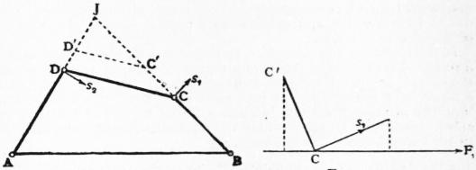
Fig. 12. Fig. 51.

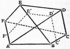
Fig. 52.

Consider, for example, a frame whose sides form the six sides of a hexagon ABCDEF and the three diagonals AD, BE, CF; and suppose that it is required to find the stress in CF due to a given system of extraneous forces in equilibrium, acting on the joints. Imagine the bar CF to be removed, and consider a deformation in which AB is fixed. The instantaneous centre of CD will be at the intersection of AD, BC, and if C′D′ be drawn parallel to CD, the lines CC′, DD′ may be taken to represent the virtual velocities of C, D turned each through a right angle. Moreover, if we draw D′E′ parallel to DE, and E′F′ parallel to EF, the lines CC′, DD′, EE′, FF′ will represent on the same scale the virtual velocities of the points C, D, E, F, respectively, turned each through a right angle. The equation of virtual work is then formed by taking moments about C′, D′, E′, F′ of the extraneous forces which act at C, D, E, F, respectively. Amongst these forces we must include the two equal and opposite forces S which take the place of the stress in the removed bar FC.

The above method lends itself naturally to the investigation of the critical forms of a frame whose general structure is given. We have seen that the stresses produced by an equilibrating system of extraneous forces in a frame which is just rigid, according to the criterion of § 6, are in general uniquely determinate; in particular, when there are no extraneous forces the bars are in general free from stress. It may however happen that owing to some special relation between the lengths of the bars the frame admits of an infinitesimal deformation. The simplest case is that of a frame of three bars, when the three joints A, B, C fall into a straight line; a small displacement of the joint B at right angles to AC would involve changes in the lengths of AB, BC which are only of the second order of small quantities. Another example is shown in fig. 53. The graphical method leads at once to the detection of such cases. Thus in the hexagonal frame of fig. 52, if an infinitesimal deformation is possible without removing the bar CF, the instantaneous centre of CF (when AB is fixed) will be at the intersection of AF and BC, and since CC′, FF′ represent the virtual velocities of the points C, F, turned each through a right angle, C′F′ must be parallel to CF. Conversely, if this condition be satisfied, an infinitesimal deformation is possible. The result may be generalized into the statement that a frame has a critical form whenever a frame of the same structure can be designed with corresponding bars parallel, but without complete geometric similarity. In the case of fig. 52 it may be shown that an equivalent condition is that the six points A, B, C, D, E, F should lie on a conic (M. W. Crofton). This is fulfilled when the opposite sides of the hexagon are parallel, and (as a still more special case) when the hexagon is regular.

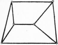
Fig. 53.

When a frame has a critical form it may be in a state of stress independently of the action of extraneous forces; moreover, the stresses due to extraneous forces are indeterminate, and may be infinite. For suppose as before that one of the bars is removed. If there are no extraneous forces the equation of virtual work reduces to S·δs = 0, where S is the stress in the removed bar, and δs is the change in the distance between the joints which it connected. In a critical form we have δs = 0, and the equation is satisfied by an arbitrary value of S; a consistent system of stresses in the remaining bars can then be found by preceding rules. Again, when extraneous forces P act on the joints, the equation is

Σ(P·δp) + S·δs = 0,

where δp is the displacement of any joint in the direction of the corresponding force P. If Σ(P·δp) = 0, the stresses are merely indeterminate as before; but if Σ (P·δp) does not vanish, the equation cannot be satisfied by any finite value of S, since δs = 0. This means that, if the material of the frame were absolutely unyielding, no finite stresses in the bars would enable it to withstand the extraneous forces. With actual materials, the frame would yield elastically, until its configuration is no longer “critical.” The stresses in the bars would then be comparatively very great, although finite. The use of frames which approximate to a critical form is of course to be avoided in practice.

A brief reference must suffice to the theory of three dimensional frames. This is important from a technical point of view, since all structures are practically three-dimensional. We may note that a frame of n joints which is just rigid must have 3n − 6 bars; and that the stresses produced in such a frame by a given system of extraneous forces in equilibrium are statically determinate, subject to the exception of “critical forms.”

§ 10. Statics of Inextensible Chains.—The theory of bodies or structures which are deformable in their smallest parts belongs properly to elasticity (q.v.). The case of inextensible strings or chains is, however, so simple that it is generally included in expositions of pure statics.

It is assumed that the form can be sufficiently represented by a plane curve, that the stress (tension) at any point P of the curve, between the two portions which meet there, is in the direction of the tangent at P, and that the forces on any linear element δs must satisfy the conditions of equilibrium laid down in § 1. It follows that the forces on any finite portion will satisfy the conditions of equilibrium which apply to the case of a rigid body (§ 4).

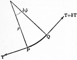
Fig. 54.

We will suppose in the first instance that the curve is plane. It is often convenient to resolve the forces on an element PQ (= δs) in the directions of the tangent and normal respectively. If T, T + δT be the tensions at P, Q, and δψ be the angle between the directions of the curve at these points, the components of the tensions along the tangent at P give (T + δT) cos ψ − T, or δT, ultimately; whilst for the component along the normal at P we have (T + δT) sin δψ, or Tδψ, or Tδs/ρ, where ρ is the radius of curvature.

Suppose, for example, that we have a light string stretched over a smooth curve; and let Rδs denote the normal pressure (outwards from the centre of curvature) on δs. The two resolutions give δT = 0, Tδψ = Rδs, or

T = const., R = T/ρ.

(1)

The tension is constant, and the pressure per unit length varies as the curvature.

Next suppose that the curve is “rough”; and let Fδs be the tangential force of friction on δs. We have δT ± Fδs = 0, Tδψ = Rδs, where the upper or lower sign is to be taken according to the sense in which F acts. We assume that in limiting equilibrium we have F = μR, everywhere, where μ is the coefficient of friction. If the string be on the point of slipping in the direction in which ψ increases, the lower sign is to be taken; hence δT = Fδs = μTδψ, whence

T = T0 eμψ,

(2)

if T0 be the tension corresponding to ψ = 0. This illustrates the resistance to dragging of a rope coiled round a post; e.g. if we put μ = .3, ψ = 2π, we find for the change of tension in one turn T/T0 = 6.5. In two turns this ratio is squared, and so on.

Again, take the case of a string under gravity, in contact with a smooth curve in a vertical plane. Let ψ denote the inclination to the horizontal, and wδs the weight of an element δs. The tangential and normal components of wδs are −s sinψ and −wδs cosψ. Hence

δT = wδs sin ψ, Tδψ = wδs cos ψ + Rδs.

(3)

If we take rectangular axes Ox, Oy, of which Oy is drawn vertically upwards, we have δy = sin ψ δs, whence δT = wδy. If the string be uniform, w is constant, and

T = wy + const. = w (y − y0),

(4)

say; hence the tension varies as the height above some fixed level (y0). The pressure is then given by the formula

R = T dψ −w cos ψ.

ds

(5)

In the case of a chain hanging freely under gravity it is usually convenient to formulate the conditions of equilibrium of a finite portion PQ. The forces on this reduce to three, viz. the weight of PQ and the tensions at P, Q. Hence these three forces will be concurrent, and their ratios will be given by a triangle of forces. In particular, if we consider a length AP beginning at the lowest point A, then resolving horizontally and vertically we have

T cos ψ = T0, T sinψ = W,

(6)

where T0 is the tension at A, and W is the weight of PA. The former equation expresses that the horizontal tension is constant.

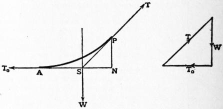
Fig. 55.

If the chain be uniform we have W = ws, where s is the arc AP: hence ws = T0 tan ψ. If we write T0 = wa, so that a is the length of a portion of the chain whose weight would equal the horizontal tension, this becomes

s = a tan ψ.

(7)

This is the “intrinsic” equation of the curve. If the axes of x and y be taken horizontal and vertical (upwards), we derive

x = a log (sec ψ + tan ψ), y = a sec ψ.

(8)

Eliminating ψ we obtain the Cartesian equation

y = a cosh x

a

(9)

of the common catenary, as it is called (fig. 56). The omission of the additive arbitrary constants of integration in (8) is equivalent to a special choice of the origin O of co-ordinates; viz. O is at a distance a vertically below the lowest point (ψ = 0) of the curve. The horizontal line through O is called the directrix. The relations

s = a sinh x , y2 = a2 + s2, T = T0 sec ψ = wy,

a

(10)

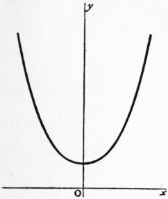
Fig. 56.

which are involved in the preceding formulae are also noteworthy. It is a classical problem in the calculus of variations to deduce the equation (9) from the condition that the depth of the centre of gravity of a chain of given length hanging between fixed points must be stationary (§ 9). The length a is called the parameter of the catenary; it determines the scale of the curve, all catenaries being geometrically similar. If weights be suspended from various points of a hanging chain, the intervening portions will form arcs of equal catenaries, since the horizontal tension (wa) is the same for all. Again, if a chain pass over a perfectly smooth peg, the catenaries in which it hangs on the two sides, though usually of different parameters, will have the same directrix, since by (10) y is the same for both at the peg.

As an example of the use of the formulae we may determine the maximum span for a wire of given material. The condition is that the tension must not exceed the weight of a certain length λ of the wire. At the ends we shall have y = λ, or

λ = a cosh x ,

a

(11)

and the problem is to make x a maximum for variations of a. Differentiating (11) we find that, if dx/da = 0,

x tanh x = 1.

a a

(12)

It is easily seen graphically, or from a table of hyperbolic tangents, that the equation u tanh u = 1 has only one positive root (u = 1.200); the span is therefore

2x = 2au = 2λ/sinh u = 1.326 λ,

and the length of wire is

2s = 2λ/u = 1.667 λ.

The tangents at the ends meet on the directrix, and their inclination to the horizontal is 56° 30′.

Fig. 57.

The relation between the sag, the tension, and the span of a wire (e.g. a telegraph wire) stretched nearly straight between two points A, B at the same level is determined most simply from first principles. If T be the tension, W the total weight, k the sag in the middle, and ψ the inclination to the horizontal at A or B, we have 2Tψ = W, AB = 2ρψ, approximately, where ρ is the radius of curvature. Since 2kρ = (1⁄2AB)2, ultimately, we have

k = 1⁄8W · AB/T.

(13)

The same formula applies if A, B be at different levels, provided k be the sag, measured vertically, half way between A and B.

In relation to the theory of suspension bridges the case where the weight of any portion of the chain varies as its horizontal projection is of interest. The vertical through the centre of gravity of the arc AP (see fig. 55) will then bisect its horizontal projection AN; hence if PS be the tangent at P we shall have AS = SN. This property is characteristic of a parabola whose axis is vertical. If we take A as origin and AN as axis of x, the weight of AP may be denoted by wx, where w is the weight per unit length at A. Since PNS is a triangle of forces for the portion AP of the chain, we have wx/T0 = PN/NS, or

y = w · x2/2T0,

(14)

which is the equation of the parabola in question. The result might of course have been inferred from the theory of the parabolic funicular in § 2.

Finally, we may refer to the catenary of uniform strength, where the cross-section of the wire (or cable) is supposed to vary as the tension. Hence w, the weight per foot, varies as T, and we may write T = wλ, where λ is a constant length. Resolving along the normal the forces on an element δs, we find Tδψ = wδs cos ψ, whence

ρ = ds = λ sec ψ.

dψ

(15)

From this we derive

x = λψ, y = λ log sec x ,

λ

(16)

where the directions of x and y are horizontal and vertical, and the origin is taken at the lowest point. The curve (fig. 58) has two vertical asymptotes x = ± 1⁄2πλ; this shows that however the thickness of a cable be adjusted there is a limit πλ to the horizontal span, where λ depends on the tensile strength of the material. For a uniform catenary the limit was found above to be 1.326λ.

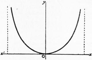
Fig. 58.

For investigations relating to the equilibrium of a string in three dimensions we must refer to the textbooks. In the case of a string stretched over a smooth surface, but in other respects free from extraneous force, the tensions at the ends of a small element δs must be balanced by the normal reaction of the surface. It follows that the osculating plane of the curve formed by the string must contain the normal to the surface, i.e. the curve must be a “geodesic,” and that the normal pressure per unit length must vary as the principal curvature of the curve.

§ 11. Theory of Mass-Systems.—This is a purely geometrical subject. We consider a system of points P1, P2 ..., Pn, with which are associated certain coefficients m1, m2, ... mn, respectively. In the application to mechanics these coefficients are the masses of particles situate at the respective points, and are therefore all positive. We shall make this supposition in what follows, but it should be remarked that hardly any difference is made in the theory if some of the coefficients have a different sign from the rest, except in the special case where Σ(m) = 0. This has a certain interest in magnetism.

In a given mass-system there exists one and only one point G such that

Σ(m·GP>) = 0.

(1)

For, take any point O, and construct the vector

OG> = Σ(m·OP>) .

Σ(m)

(2)

Then

Σ(m·GP>) = Σ {m(GO> + OP>)} = Σ(m)·GO> + Σ(m)·OP> = 0.

(3)

Also there cannot be a distinct point G′ such that Σ(m·G′P) = 0, for we should have, by subtraction,

Σ {m(GP> + PG>′)} = 0, or Σ(m)·GG′ = 0;

(4)

i.e. G′ must coincide with G. The point G determined by (1) is called the mass-centre or centre of inertia of the given system. It is easily seen that, in the process of determining the mass-centre, any group of particles may be replaced by a single particle whose mass is equal to that of the group, situate at the mass-centre of the group.

If through P1, P2, ... Pn we draw any system of parallel planes meeting a straight line OX in the points M1, M2 ... Mn, the collinear vectors OM>1, OM>2 ... OM>n may be called the “projections” of OP>1, OP>2, ... OP>n on OX. Let these projections be denoted algebraically by x1, x2, ... xn, the sign being positive or negative according as the direction is that of OX or the reverse. Since the projection of a vector-sum is the sum of the projections of the several vectors, the equation (2) gives

x = Σ(mx) ,

Σ(m)

(5)

if x be the projection of OG>. Hence if the Cartesian co-ordinates of P1, P2, ... Pn relative to any axes, rectangular or oblique be (x1, y1, z1), (x2, y2, z2), ..., (xn, yn, zn), the mass-centre (x, y, z) is determined by the formulae

x = Σ(mx) , y = Σ(my) , z = Σ(mz) .

Σ(m) Σ(m) Σ(m)

(6)

If we write x = x + ξ, y = y + η, z = z + ζ, so that ξ, η, ζ denote co-ordinates relative to the mass-centre G, we have from (6)

Σ(mξ) = 0, Σ(mη) = 0, Σ(mζ) = 0.

(7)

One or two special cases may be noticed. If three masses α, β, γ be situate at the vertices of a triangle ABC, the mass-centre of β and γ is at a point A′ in BC, such that β·BA′ = γ·A′C. The mass-centre (G) of α, β, γ will then divide AA′ so that α·AG = (β + γ) GA′. It is easily proved that

α : β : γ = ΔBGA : ΔGCA : ΔGAB;

also, by giving suitable values (positive or negative) to the ratios α : β : γ we can make G assume any assigned position in the plane ABC. We have here the origin of the “barycentric co-ordinates” of Möbius, now usually known as “areal” co-ordinates. If α + β + γ = 0, G is at infinity; if α = β = γ, G is at the intersection of the median lines of the triangle; if α : β : γ = a : b : c, G is at the centre of the inscribed circle. Again, if G be the mass-centre of four particles α, β, γ, δ situate at the vertices of a tetrahedron ABCD, we find

α : β : γ : δ = tetn GBCD : tetn GCDA : tetn GDAB : tetn GABC,

and by suitable determination of the ratios on the left hand we can make G assume any assigned position in space. If α + β + γ + δ = O, G is at infinity; if α = β = γ = δ, G bisects the lines joining the middle points of opposite edges of the tetrahedron ABCD; if α : β : γ : δ = ΔBCD : ΔCDA : ΔDAB : ΔABC, G is at the centre of the inscribed sphere.

If we have a continuous distribution of matter, instead of a system of discrete particles, the summations in (6) are to be replaced by integrations. Examples will be found in textbooks of the calculus and of analytical statics. As particular cases: the mass-centre of a uniform thin triangular plate coincides with that of three equal particles at the corners; and that of a uniform solid tetrahedron coincides with that of four equal particles at the vertices. Again, the mass-centre of a uniform solid right circular cone divides the axis in the ratio 3 : 1; that of a uniform solid hemisphere divides the axial radius in the ratio 3 : 5.

It is easily seen from (6) that if the configuration of a system of particles be altered by “homogeneous strain” (see Elasticity) the new position of the mass-centre will be at that point of the strained figure which corresponds to the original mass-centre.

The formula (2) shows that a system of concurrent forces represented by m1·OP>1, m2·OP>2, ... mn·OP>n will have a resultant represented hy Σ(m)·OG>. If we imagine O to recede to infinity in any direction we learn that a system of parallel forces proportional to m1, m2,... mn, acting at P1, P2 ... Pn have a resultant proportional to Σ(m) which acts always through a point G fixed relatively to the given mass-system. This contains the theory of the “centre of gravity” (§§ 4, 9). We may note also that if P1, P2, ... Pn, and P1′, P2′, ... Pn′ represent two configurations of the series of particles, then

Σ(m·PP>′) = Sigma(m)·GG>′,

(8)

where G, G′ are the two positions of the mass-centre. The forces m1·P>1P1′, m2·P>2P2′, ... mn·P>nPn′, considered as localized vectors, do not, however, as a rule reduce to a single resultant.

We proceed to the theory of the plane, axial and polar quadratic moments of the system. The axial moments have alone a dynamical significance, but the others are useful as subsidiary conceptions. If h1, h2, ... hn be the perpendicular distances of the particles from any fixed plane, the sum Σ(mh2) is the quadratic moment with respect to the plane. If p1, p2, ... pn be the perpendicular distances from any given axis, the sum Σ(mp2) is the quadratic moment with respect to the axis; it is also called the moment of inertia about the axis. If r1, r2, ... rn be the distances from a fixed point, the sum Σ(mr2) is the quadratic moment with respect to that point (or pole). If we divide any of the above quadratic moments by the total mass Σ(m), the result is called the mean square of the distances of the particles from the respective plane, axis or pole. In the case of an axial moment, the square root of the resulting mean square is called the radius of gyration of the system about the axis in question. If we take rectangular axes through any point O, the quadratic moments with respect to the co-ordinate planes are

Ix = Σ(mx2), Iy = Σ(my2), Iz = Σ(mz2);

(9)

those with respect to the co-ordinate axes are

Iyz = Σ {m (y2 + z2)}, Izx = Σ {m (z2 + x2)}, Ixy = Σ {m (x2 + y2)};

(10)

whilst the polar quadratic moment with respect to O is

I0 = Σ {m (x2 + y2 + z2)}.

(11)

We note that

Iyz = Iy + Iz, Izx = Iz + Ix, Ixy = Ix + Iy,

(12)

and

I0 = Ix + Iy + Iz = 1⁄2 (Iyz + Izx + Ixy).

(13)

In the case of continuous distributions of matter the summations in (9), (10), (11) are of course to be replaced by integrations. For a uniform thin circular plate, we find, taking the origin at its centre, and the axis of z normal to its plane, I0 = 1⁄2Ma2, where M is the mass and a the radius. Since Ix = Iy, Iz = 0, we deduce Izx = 1⁄2Ma2, Ixy = 1⁄2Ma2; hence the value of the squared radius of gyration is for a diameter 1⁄4a2, and for the axis of symmetry 1⁄2a2. Again, for a uniform solid sphere having its centre at the origin we find I0 = 3⁄5Ma2, Ix = Iy = Iz = 1⁄5Ma2, Iyz = Izx = lxy = 3⁄5Ma2; i.e. the square of the radius of gyration with respect to a diameter is 2⁄5a2. The method of homogeneous strain can be applied to deduce the corresponding results for an ellipsoid of semi-axes a, b, c. If the co-ordinate axes coincide with the principal axes, we find Ix = 1⁄5Ma2, Iy = 1⁄5Mb2, Iz = 1⁄5Mc2, whence Iyz = 1⁄5M (b2 + c2), &c.

If φ(x, y, z) be any homogeneous quadratic function of x, y, z, we have

Σ {mφ (x, y, z)} = Σ {mφ (x + ξ, y + η, z + ζ) } = Σ {mφ (x, y, z)} + Σ {mφ (ξ, η, ζ)},

(14)

since the terms which are bilinear in respect to x, y, z, and ξ, η, ζ vanish, in virtue of the relations (7). Thus

Ix = Iξ + Σ(m)x2,

(15)

Iyz = Iηζ + Σ(m) · (y2 + z2),

(16)

with similar relations, and

IO = IG + Σ(m) · OG2.

(17)

The formula (16) expresses that the squared radius of gyration about any axis (Ox) exceeds the squared radius of gyration about a parallel axis through G by the square of the distance between the two axes. The formula (17) is due to J. L. Lagrange; it may be written

Σ(m · OP2) = Σ(m · GP2) + OG2,

Σ(m) Σ(m)

(18)

and expresses that the mean square of the distances of the particles from O exceeds the mean square of the distances from G by OG2. The mass-centre is accordingly that point the mean square of whose distances from the several particles is least. If in (18) we make O coincide with P1, P2, ... Pn in succession, we obtain

0 + m2·P1P22 + ... + mn·P1Pn2 = Σ(m · GP2) + Σ(m) · GP12,

m1·P2P12 + 0 + ... + mn·P2Pn2 = Σ(m · GP2) + Σ(m) · GP22,

.........

m1·PnP12 + m2·PnP22 + ... + 0 = Σ(m · GP2) + Σ(m) · GPn2.

(19)

If we multiply these equations by m1, m2 ... mn, respectively, and add, we find

ΣΣ (mrms · PrPs2) = Σ (m) · Σ (m · GP2),

(20)

provided the summation ΣΣ on the left hand be understood to include each pair of particles once only. This theorem, also due to Lagrange, enables us to express the mean square of the distances of the particles from the centre of mass in terms of the masses and mutual distances. For instance, considering four equal particles at the vertices of a regular tetrahedron, we can infer that the radius R of the circumscribing sphere is given by R2 = 3⁄8a2, if a be the length of an edge.

Another type of quadratic moment is supplied by the deviation-moments, or products of inertia of a distribution of matter. Thus the sum Σ(m·yz) is called the “product of inertia” with respect to the planes y = 0, z = 0. This may be expressed In terms of the product of inertia with respect to parallel planes through G by means of the formula (14); viz.:—

Σ (m · yz) = Σ (m · ηζ) + Σ (m) · yz

(21)

The quadratic moments with respect to different planes through a fixed point O are related to one another as follows. The moment with respect to the plane

λx + μy + νz = 0,

(22)

where λ, μ, ν are direction-cosines, is

Σ {m (λx + μy + νz)2} = Σ (mx2)·λ2 + Σ (my2)·μ2 + Σ (mz2)·ν2 + 2Σ (myz)·μν + 2Σ (mzx)·νλ + 2Σ (mxy)·λμ,

(23)

and therefore varies as the square of the perpendicular drawn from O to a tangent plane of a certain quadric surface, the tangent plane in question being parallel to (22). If the co-ordinate axes coincide with the principal axes of this quadric, we shall have

Σ(myz) = 0, Σ(mzx) = 0, Σ(mxy) = 0;

(24)

and if we write

Σ(mx2) = Ma2, Σ(my2) = Mb2, Σ(mz2) = Mc2,

(25)

where M = Σ(m), the quadratic moment becomes M(a2λ2 + b2μ2 + c2ν2), or Mp2, where p is the distance of the origin from that tangent plane of the ellipsoid

x2 + y2 + z2 = 1,

a2 b2 c2

(26)

which is parallel to (22). It appears from (24) that through any assigned point O three rectangular axes can be drawn such that the product of inertia with respect to each pair of co-ordinate planes vanishes; these are called the principal axes of inertia at O. The ellipsoid (26) was first employed by J. Binet (1811), and may be called “Binet’s Ellipsoid” for the point O. Evidently the quadratic moment for a variable plane through O will have a “stationary” value when, and only when, the plane coincides with a principal plane of (26). It may further be shown that if Binet’s ellipsoid be referred to any system of conjugate diameters as co-ordinate axes, its equation will be

x′2 + y′2 + z′2 = 1,

a′2 b′2 c′2

(27)

provided

Σ(mx′2) = Ma′2, Σ(my′2) Mb′2, Σ(mz′2) = Mc′2;

also that

Σ(my′z′) = 0, Σ(mz′x′) = 0, Σ(mx′y′) = 0.

(28)

Let us now take as co-ordinate axes the principal axes of inertia at the mass-centre G. If a, b, c be the semi-axes of the Binet’s ellipsoid of G, the quadratic moment with respect to the plane λx + μy + νz = 0 will be M(a2λ2 + b2μ2 + c2ν2), and that with respect to a parallel plane

λx + μy + νz = p

(29)

will be M (a2λ2 + b2μ2 + c2ν2 + p2), by (15). This will have a given value Mk2, provided

p2 = (k2 − a2) λ2 + (k2 − b2) μ2 + (k2 − c2) ν2.

(30)

Hence the planes of constant quadratic moment Mk2 will envelop the quadric

x2 + y2 + z2 = 1,

k2 − a2 k2 − b2 k2 − c2

(31)

and the quadrics corresponding to different values of k2 will be confocal. If we write

k2 = a2 + b2 + c2 + θ, b2 + c2 = α2, c2 + a2 = β2, a2 + b2 = γ2

(32)

the equation (31) becomes

x2 + y2 + z2 = 1;

α2 + θ β2 + θ γ2 + θ

(33)

for different values of θ this represents a system of quadrics confocal with the ellipsoid

x2 + y2 + z2 = 1,

α2 β2 γ2

(34)

which we shall meet with presently as the “ellipsoid of gyration” at G. Now consider the tangent plane ω at any point P of a confocal, the tangent plane ω′ at an adjacent point N′, and a plane ω″ through P parallel to ω′. The distance between the planes ω′ and ω″ will be of the second order of small quantities, and the quadratic moments with respect to ω′ and ω″ will therefore be equal, to the first order. Since the quadratic moments with respect to ω and ω′ are equal, it follows that ω is a plane of stationary quadratic moment at P, and therefore a principal plane of inertia at P. In other words, the principal axes of inertia at P arc the normals to the three confocals of the system (33) which pass through P. Moreover if x, y, z be the co-ordinates of P, (33) is an equation to find the corresponding values of θ; and if θ1, θ2, θ3 be the roots we find

θ1 + θ2 + θ3 = r2 − α2 − β2 − γ2,

(35)

where r2 = x2 + y2 + z2. The squares of the radii of gyration about the principal axes at P may be denoted by k22 + k32, k32 + k12, k12 + k22; hence by (32) and (35) they are r2 −θ1, r2 − θ2, r2 − θ3, respectively.

To find the relations between the moments of inertia about different axes through any assigned point O, we take O as origin. Since the square of the distance of a point (x, y, z) from the axis

x = y = z

λ μ ν

(36)

is x2 + y2 + z2 − (λx + μy + νz)2, the moment of inertia about this axis is

I = Σ [m { (λ2 + μ2 + ν2) (x2 + y2 + z2) − (λx + μy + νz)2} ] = Aλ2 + Bμ2 + Cν2 − 2Fμν − 2Gνλ − 2Hλμ,

(37)

provided

A = Σ {m (y2 + z2)}, B = Σ {m (z2 + x2)}, C = Σ {m (x2 + y2)}, F = Σ (myz), G = Σ (mzx), H = Σ (mxy);

(38)

i.e. A, B, C are the moments of inertia about the co-ordinate axes, and F, G, H are the products of inertia with respect to the pairs of co-ordinate planes. If we construct the quadric

Ax2 + By2 + Cz2 − 2Fyz − 2Gzx − 2Hxy = Mε4

(39)

where ε is an arbitrary linear magnitude, the intercept r which it makes on a radius drawn in the direction λ, μ, ν is found by putting x, y, z = λr, μr, νr. Hence, by comparison with (37),

I = Mε4 / r2.

(40)

The moment of inertia about any radius of the quadric (39) therefore varies inversely as the square of the length of this radius. When referred to its principal axes, the equation of the quadric takes the form

Ax2 + By2 + Cz2 = Mε4.

(41)

The directions of these axes are determined by the property (24), and therefore coincide with those of the principal axes of inertia at O, as already defined in connexion with the theory of plane quadratic moments. The new A, B, C are called the principal moments of inertia at O. Since they are essentially positive the quadric is an ellipsoid; it is called the momental ellipsoid at O. Since, by (12), B + C > A, &c., the sum of the two lesser principal moments must exceed the greatest principal moment. A limitation is thus imposed on the possible forms of the momental ellipsoid; e.g. in the case of symmetry about an axis it appears that the ratio of the polar to the equatorial diameter of the ellipsoid cannot be less than 1/√2.

If we write A = Mα2, B = Mβ2, C = Mγ2, the formula (37), when referred to the principal axes at O, becomes

I = M (α2λ2 + β2μ2 + γ2ν2) = Mp2,

(42)

if p denotes the perpendicular drawn from O in the direction (λ, μ, ν) to a tangent plane of the ellipsoid

x2 + y2 + z2 = 1

α2 β2 γ2

(43)

This is called the ellipsoid of gyration at O; it was introduced into the theory by J. MacCullagh. The ellipsoids (41) and (43) are reciprocal polars with respect to a sphere having O as centre.

If A = B = C, the momental ellipsoid becomes a sphere; all axes through O are then principal axes, and the moment of inertia is the same for each. The mass-system is then said to possess kinetic symmetry about O.

If all the masses lie in a plane (z = 0) we have, in the notation of (25), c2 = 0, and therefore A = Mb2, B = Ma2, C = M(a2 + b2), so that the equation of the momental ellipsoid takes the form

b2x2 + a2y2 + (a2 + b2) z2 = ε4.

(44)

The section of this by the plane z = 0 is similar to

x2 + y2 = 1,

a2 b2

(45)

which may be called the momental ellipse at O. It possesses the property that the radius of gyration about any diameter is half the distance between the two tangents which are parallel to that diameter. In the case of a uniform triangular plate it may be shown that the momental ellipse at G is concentric, similar and similarly situated to the ellipse which touches the sides of the triangle at their middle points.

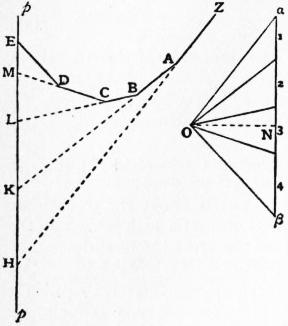
Fig. 59.

The graphical methods of determining the moment of inertia of a plane system of particles with respect to any line in its plane may be briefly noticed. It appears from § 5 (fig. 31) that the linear moment of each particle about the line may be found by means of a funicular polygon. If we replace the mass of each particle by its moment, as thus found, we can in like manner obtain the quadratic moment of the system with respect to the line. For if the line in question be the axis of y, the first process gives us the values of mx, and the second the value of Σ(mx·x) or Σ(mx2). The construction of a second funicular may be dispensed with by the employment of a planimeter, as follows. In fig. 59 p is the line with respect to which moments are to be taken, and the masses of the respective particles are indicated by the corresponding segments of a line in the force-diagram, drawn parallel to p. The funicular ZABCD ... corresponding to any pole O is constructed for a system of forces acting parallel to p through the positions of the particles and proportional to the respective masses; and its successive sides are produced to meet p in the points H, K, L, M, ... As explained in § 5, the moment of the first particle is represented on a certain scale by HK, that of the second by KL, and so on. The quadratic moment of the first particle will then be represented by twice the area AHK, that of the second by twice the area BKL, and so on. The quadratic moment of the whole system is therefore represented by twice the area AHEDCBA. Since a quadratic moment is essentially positive, the various areas are to taken positive in all cases. If k be the radius of gyration about p we find

k2 = 2 × area AHEDCBA × ON ÷ αβ,

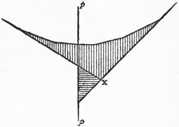
Fig. 60.

where αβ is the line in the force-diagram which represents the sum of the masses, and ON is the distance of the pole O from this line. If some of the particles lie on one side of p and some on the other, the quadratic moment of each set may be found, and the results added. This is illustrated in fig. 60, where the total quadratic moment is represented by the sum of the shaded areas. It is seen that for a given direction of p this moment is least when p passes through the intersection X of the first and last sides of the funicular; i.e. when p goes through the mass-centre of the given system; cf. equation (15).

Part II.—Kinetics

§ 12. Rectilinear Motion.—Let x denote the distance OP of a moving point P at time t from a fixed origin O on the line of motion, this distance being reckoned positive or negative according as it lies to one side or the other of O. At time t + δt let the point be at Q, and let OQ = x + δx. The mean velocity of the point in the interval δt is δx/δt. The limiting value of this when δt is infinitely small, viz. dx/dt, is adopted as the definition of the velocity at the instant t. Again, let u be the velocity at time t, u + δu that at time t + δt. The mean rate of increase of velocity, or the mean acceleration, in the interval δt is then δu/δt. The limiting value of this when δt is infinitely small, viz., du/dt, is adopted as the definition of the acceleration at the instant t. Since u = dx/dt, the acceleration is also denoted by d2x/dt2. It is often convenient to use the “fluxional” notation for differential coefficients with respect to time; thus the velocity may be represented by ẋ and the acceleration by u̇ or ẍ. There is another formula for the acceleration, in which u is regarded as a function of the position; thus du/dt = (du/dx) (dx/dt) = u(du/dx). The relation between x and t in any particular case may be illustrated by means of a curve constructed with t as abscissa and x as ordinate. This is called the curve of positions or space-time curve; its gradient represents the velocity. Such curves are often traced mechanically in acoustical and other experiments. A, curve with t as abscissa and u as ordinate is called the curve of velocities or velocity-time curve. Its gradient represents the acceleration, and the area (∫u dt) included between any two ordinates represents the space described in the interval between the corresponding instants (see fig. 62).

So far nothing has been said about the measurement of time. From the purely kinematic point of view, the t of our formulae may be any continuous independent variable, suggested (it may be) by some physical process. But from the dynamical standpoint it is obvious that equations which represent the facts correctly on one system of time-measurement might become seriously defective on another. It is found that for almost all purposes a system of measurement based ultimately on the earth’s rotation is perfectly adequate. It is only when we come to consider such delicate questions as the influence of tidal friction that other standards become necessary.

The most important conception in kinetics is that of “inertia.” It is a matter of ordinary observation that different bodies acted on by the same force, or what is judged to be the same force, undergo different changes of velocity in equal times. In our ideal representation of natural phenomena this is allowed for by endowing each material particle with a suitable mass or inertia-coefficient m. The product mu of the mass into the velocity is called the momentum or (in Newton’s phrase) the quantity of motion. On the Newtonian system the motion of a particle entirely uninfluenced by other bodies, when referred to a suitable base, would be rectilinear, with constant velocity. If the velocity changes, this is attributed to the action of force; and if we agree to measure the force (X) by the rate of change of momentum which it produces, we have the equation

d (mu) = X.

dt

(1)

From this point of view the equation is a mere truism, its real importance resting on the fact that by attributing suitable values to the masses m, and by making simple assumptions as to the value of X in each case, we are able to frame adequate representations of whole classes of phenomena as they actually occur. The question remains, of course, as to how far the measurement of force here implied is practically consistent with the gravitational method usually adopted in statics; this will be referred to presently.

The practical unit or standard of mass must, from the nature of the case, be the mass of some particular body, e.g. the imperial pound, or the kilogramme. In the “C.G.S.” system a subdivision of the latter, viz. the gramme, is adopted, and is associated with the centimetre as the unit of length, and the mean solar second as the unit of time. The unit of force implied in (1) is that which produces unit momentum in unit time. On the C.G.S. system it is that force which acting on one gramme for one second produces a velocity of one centimetre per second; this unit is known as the dyne. Units of this kind are called absolute on account of their fundamental and invariable character as contrasted with gravitational units, which (as we shall see presently) vary somewhat with the locality at which the measurements are supposed to be made.

If we integrate the equation (1) with respect to t between the limits t, t′ we obtain

mu′ − mu = ∫t′t X dt.

(2)

The time-integral on the right hand is called the impulse of the force on the interval t′ − t. The statement that the increase of momentum is equal to the impulse is (it maybe remarked) equivalent to Newton’s own formulation of his Second Law. The form (1) is deduced from it by putting t′ − t = δt, and taking δt to be infinitely small. In problems of impact we have to deal with cases of practically instantaneous impulse, where a very great and rapidly varying force produces an appreciable change of momentum in an exceedingly minute interval of time.

In the case of a constant force, the acceleration u̇ or ẍ is, according to (1), constant, and we have

d2x = α,

dt2

(3)

say, the general solution of which is

x = 1⁄2 αt2 + At + B.

(4)

The “arbitrary constants” A, B enable us to represent the circumstances of any particular case; thus if the velocity ẋ and the position x be given for any one value of t, we have two conditions to determine A, B. The curve of positions corresponding to (4) is a parabola, and that of velocities is a straight line. We may take it as an experimental result, although the best evidence is indirect, that a particle falling freely under gravity experiences a constant acceleration which at the same place is the same for all bodies. This acceleration is denoted by g; its value at Greenwich is about 981 centimetre-second units, or 32.2 feet per second. It increases somewhat with the latitude, the extreme variation from the equator to the pole being about 1⁄2%. We infer that on our reckoning the force of gravity on a mass m is to be measured by mg, the momentum produced per second when this force acts alone. Since this is proportional to the mass, the relative masses to be attributed to various bodies can be determined practically by means of the balance. We learn also that on account of the variation of g with the locality a gravitational system of force-measurement is inapplicable when more than a moderate degree of accuracy is desired.

We take next the case of a particle attracted towards a fixed point O in the line of motion with a force varying as the distance from that point. If μ be the acceleration at unit distance, the equation of motion becomes

d2x = −μx,

dt2

(5)

the solution of which may be written in either of the forms

x = A cos σt + B sin σt, x = a cos (σt + ε),

(6)

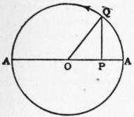
Fig. 61.

where σ= √μ, and the two constants A, B or a, ε are arbitrary. The particle oscillates between the two positions x = ±a, and the same point is passed through in the same direction with the same velocity at equal intervals of time 2π/σ. The type of motion represented by (6) is of fundamental importance in the theory of vibrations (§ 23); it is called a simple-harmonic or (shortly) a simple vibration. If we imagine a point Q to describe a circle of radius a with the angular velocity σ, its orthogonal projection P on a fixed diameter AA′ will execute a vibration of this character. The angle σt + ε (or AOQ) is called the phase; the arbitrary elements a, ε are called the amplitude and epoch (or initial phase), respectively. In the case of very rapid vibrations it is usual to specify, not the period (2π/σ), but its reciprocal the frequency, i.e. the number of complete vibrations per unit time. Fig. 62 shows the curves of position and velocity; they both have the form of the “curve of sines.” The numbers correspond to an amplitude of 10 centimetres and a period of two seconds.

The vertical oscillations of a weight which hangs from a fixed point by a spiral spring come under this case. If M be the mass, and x the vertical displacement from the position of equilibrium, the equation of motion is of the form

M d2x = − Kx,

dt2

(7)

provided the inertia of the spring itself be neglected. This becomes identical with (5) if we put μ = K/M; and the period is therefore 2π√(M/K), the same for all amplitudes. The period is increased by an increase of the mass M, and diminished by an increase in the stiffness (K) of the spring. If c be the statical increase of length which is produced by the gravity of the mass M, we have Kc = Mg, and the period is 2π√(c/g).

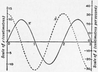
Fig. 62.

The small oscillations of a simple pendulum in a vertical plane also come under equation (5). According to the principles of § 13, the horizontal motion of the bob is affected only by the horizontal component of the force acting upon it. If the inclination of the string to the vertical does not exceed a few degrees, the vertical displacement of the particle is of the second order, so that the vertical acceleration may be neglected, and the tension of the string may be equated to the gravity mg of the particle. Hence if l be the length of the string, and x the horizontal displacement of the bob from the equilibrium position, the horizontal component of gravity is mgx/l, whence

d2x = − gx ,

dt2 l

(8)

The motion is therefore simple-harmonic, of period τ = 2π√(l/g). This indicates an experimental method of determining g with considerable accuracy, using the formula g = 4π2l/τ2.

In the case of a repulsive force varying as the distance from the origin, the equation of motion is of the type

d2x = μx,

dt2

(9)

the solution of which is

x = Aent + Be−nt,

(10)

where n = √μ. Unless the initial conditions be adjusted so as to make A = 0 exactly, x will ultimately increase indefinitely with t. The position x = 0 is one of equilibrium, but it is unstable. This applies to the inverted pendulum, with μ = g/l, but the equation (9) is then only approximate, and the solution therefore only serves to represent the initial stages of a motion in the neighbourhood of the position of unstable equilibrium.

In acoustics we meet with the case where a body is urged towards a fixed point by a force varying as the distance, and is also acted upon by an “extraneous” or “disturbing” force which is a given function of the time. The most important case is where this function is simple-harmonic, so that the equation (5) is replaced by

d2x + μx = ƒ cos (σ1t + α),

dt2

(11)

where σ1 is prescribed. A particular solution is

x = ƒ cos (σ1t + α).

μ − σ12

(12)

This represents a forced oscillation whose period 2π/σ1, coincides with that of the disturbing force; and the phase agrees with that of the force, or is opposed to it, according as σ12 < or > μ; i.e. according as the imposed period is greater or less than the natural period 2π/√μ. The solution fails when the two periods agree exactly; the formula (12) is then replaced by

x = ƒt sin (σ1t + α),

2σ1

(13)

which represents a vibration of continually increasing amplitude. Since the equation (12) is in practice generally only an approximation (as in the case of the pendulum), this solution can only be accepted as a representation of the initial stages of the forced oscillation. To obtain the complete solution of (11) we must of course superpose the free vibration (6) with its arbitrary constants in order to obtain a complete representation of the most general motion consequent on arbitrary initial conditions.

A simple mechanical illustration is afforded by the pendulum. If the point of suspension have an imposed simple vibration ξ = a cos σt in a horizontal line, the equation of small motion of the bob is

mẍ = −mg x − ξ ,

l

or

ẍ + gx = g ξ .

l l

(14)

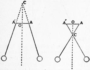
Fig. 63.

This is the same as if the point of suspension were fixed, and a horizontal disturbing force mgξ/l were to act on the bob. The difference of phase of the forced vibration in the two cases is illustrated and explained in the annexed fig. 63, where the pendulum virtually oscillates about C as a fixed point of suspension. This illustration was given by T. Young in connexion with the kinetic theory of the tides, where the same point arises.

We may notice also the case of an attractive force varying inversely as the square of the distance from the origin. If μ be the acceleration at unit distance, we have

u du = − μ

dx x2

(15)

whence

u2 = 2μ + C.

x

(16)

In the case of a particle falling directly towards the earth from rest at a very great distance we have C = 0 and, by Newton’s Law of Gravitation, μ/a2 = g, where a is the earth’s radius. The deviation of the earth’s figure from sphericity, and the variation of g with latitude, are here ignored. We find that the velocity with which the particle would arrive at the earth’s surface (x = a) is √(2ga). If we take as rough values a = 21 × 106 feet, g = 32 foot-second units, we get a velocity of 36,500 feet, or about seven miles, per second. If the particles start from rest at a finite distance c, we have in (16), C = − 2μ/c, and therefore

dx = u = − √ { 2μ (c − x) },

dt cx

(17)

the minus sign indicating motion towards the origin. If we put x = c cos2 1⁄2φ, we find

t = c3/2 (φ + sin φ),

√(8μ)

(18)

no additive constant being necessary if t be reckoned from the instant of starting, when φ = 0. The time t of reaching the origin (φ = π) is

t1 = π c3/2 .

√(8μ)

(19)

This may be compared with the period of revolution in a circular orbit of radius c about the same centre of force, viz. 2πc3/2 / √μ (§ 14). We learn that if the orbital motion of a planet, or a satellite, were arrested, the body would fall into the sun, or into its primary, in the fraction 0.1768 of its actual periodic time. Thus the moon would reach the earth in about five days. It may be noticed that if the scales of x and t be properly adjusted, the curve of positions in the present problem is the portion of a cycloid extending from a vertex to a cusp.

In any case of rectilinear motion, if we integrate both sides of the equation

mu du = X,

dx

(20)

which is equivalent to (1), with respect to x between the limits x0, x1, we obtain

1⁄2 mu12 − 1⁄2 mu02 = ∫x1x0 X dx.

(21)

We recognize the right-hand member as the work done by the force X on the particle as the latter moves from the position x0 to the position x1. If we construct a curve with x as abscissa and X as ordinate, this work is represented, as in J. Watt’s “indicator-diagram,” by the area cut off by the ordinates x = x0, x = x1. The product 1⁄2mu2 is called the kinetic energy of the particle, and the equation (21) is therefore equivalent to the statement that the increment of the kinetic energy is equal to the work done on the particle. If the force X be always the same in the same position, the particle may be regarded as moving in a certain invariable “field of force.” The work which would have to be supplied by other forces, extraneous to the field, in order to bring the particle from rest in some standard position P0 to rest in any assigned position P, will depend only on the position of P; it is called the statical or potential energy of the particle with respect to the field, in the position P. Denoting this by V, we have δV − Xδx = 0, whence

X = − dV .

dx

(22)

The equation (21) may now be written

1⁄2 mu12 + V1 = 1⁄2 mu02 + V0,

(23)

which asserts that when no extraneous forces act the sum of the kinetic and potential energies is constant. Thus in the case of a weight hanging by a spiral spring the work required to increase the length by x is V = ∫x0 Kx dx = 1⁄2Kx2, whence 1⁄2Mu2 + 1⁄2Kx2 = const., as is easily verified from preceding results. It is easily seen that the effect of extraneous forces will be to increase the sum of the kinetic and potential energies by an amount equal to the work done by them. If this amount be negative the sum in question is diminished by a corresponding amount. It appears then that this sum is a measure of the total capacity for doing work against extraneous resistances which the particle possesses in virtue of its motion and its position; this is in fact the origin of the term “energy.” The product mv2 had been called by G. W. Leibnitz the “vis viva”; the name “energy” was substituted by T. Young; finally the name “actual energy” was appropriated to the expression 1⁄2mv2 by W. J. M. Rankine.

The laws which regulate the resistance of a medium such as air to the motion of bodies through it are only imperfectly known. We may briefly notice the case of resistance varying as the square of the velocity, which is mathematically simple. If the positive direction of x be downwards, the equation of motion of a falling particle will be of the form

du = g − ku2;

dt

(24)

this shows that the velocity u will send asymptotically to a certain limit V (called the terminal velocity) such that kV2 = g. The solution is

u = V tanh gt , x = V2 log cosh gt ,

V g V

(25)

if the particle start from rest in the position x = 0 at the instant t = 0. In the case of a particle projected vertically upwards we have

du = −g − ku2,

dt

(26)

the positive direction being now upwards. This leads to

tan−1 u = tan−1 u0 − gt , x = V2 log V2 + u02 ,

V V V 2g V2 + u2

(27)

where u0 is the velocity of projection. The particle comes to rest when

t = V tan−1 u0 , x = V2 log ( 1 + u02 ).

g V 2g V2

(28)

For small velocities the resistance of the air is more nearly proportional to the first power of the velocity. The effect of forces of this type on small vibratory motions may be investigated as follows. The equation (5) when modified by the introduction of a frictional term becomes

ẍ = −μx − kẋ.

(29)

If k2 < 4μ the solution is

x = a e−t/τ cos (σt + ε),

(30)

where

τ = 2/k, σ = √(μ − 1⁄4k2),

(31)

and the constants a, ε are arbitrary. This may be described as a simple harmonic oscillation whose amplitude diminishes asymptotically to zero according to the law e−t/τ. The constant τ is called the modulus of decay of the oscillations; if it is large compared with 2π/σ the effect of friction on the period is of the second order of small quantities and may in general be ignored. We have seen that a true simple-harmonic vibration may be regarded as the orthogonal projection of uniform circular motion; it was pointed out by P. G. Tait that a similar representation of the type (30) is obtained if we replace the circle by an equiangular spiral described, with a constant angular velocity about the pole, in the direction of diminishing radius vector. When k2 > 4μ, the solution of (29) is, in real form,

x = a1e−t/τ1 + a2e−t/τ2,

(32)

where

1/τ1, 1/τ2 = 1⁄2k ± √(1⁄4k2 − μ).

(33)

The body now passes once (at most) through its equilibrium position, and the vibration is therefore styled aperiodic.

To find the forced oscillation due to a periodic force we have

ẍ + kẋ + μx = ƒ cos (σ1t + ε).

(34)

The solution is

x = ƒ cos (σ1t + ε − ε1),

R

(35)

provided

R = { (μ − σ12)2 + k2σ12}1/2, tan ε1 = kσ1 .

μ − σ12

(36)

Hence the phase of the vibration lags behind that of the force by the amount ε1, which lies between 0 and 1⁄2π or between 1⁄2π and π, according as σ12 ≶ μ. If the friction be comparatively slight the amplitude is greatest when the imposed period coincides with the free period, being then equal to ƒ/kσ1, and therefore very great compared with that due to a slowly varying force of the same average intensity. We have here, in principle, the explanation of the phenomenon of “resonance” in acoustics. The abnormal amplitude is greater, and is restricted to a narrower range of frequency, the smaller the friction. For a complete solution of (34) we must of course superpose the free vibration (30); but owing to the factor e−t/τ the influence of the initial conditions gradually disappears.

For purposes of mathematical treatment a force which produces a finite change of velocity in a time too short to be appreciated is regarded as infinitely great, and the time of action as infinitely short. The whole effect is summed up in the value of the instantaneous impulse, which is the time-integral of the force. Thus if an instantaneous impulse ξ changes the velocity of a mass m from u to u′ we have

mu′ − mu = ξ.

(37)

The effect of ordinary finite forces during the infinitely short duration of this impulse is of course ignored.

We may apply this to the theory of impact. If two masses m1, m2 moving in the same straight line impinge, with the result that the velocities are changed from u1, u2, to u1′, u2′, then, since the impulses on the two bodies must be equal and opposite, the total momentum is unchanged, i.e.

m1u1′ + m2u2′ = m1u1 + m2u2.

(38)

The complete determination of the result of a collision under given circumstances is not a matter of abstract dynamics alone, but requires some auxiliary assumption. If we assume that there is no loss of apparent kinetic energy we have also

m1u1′2 + m2u2′2 = m1u12 + m2u22.

(39)

Hence, and from (38),

u2′ − u1′ = −(u2 − u1),

(40)

i.e. the relative velocity of the two bodies is reversed in direction, but unaltered in magnitude. This appears to be the case very approximately with steel or glass balls; generally, however, there is some appreciable loss of apparent energy; this is accounted for by vibrations produced in the balls and imperfect elasticity of the materials. The usual empirical assumption is that

u2′ − u1′ = −e (u2 − u1),

(41)

where e is a proper fraction which is constant for the same two bodies. It follows from the formula § 15 (10) for the internal kinetic energy of a system of particles that as a result of the impact this energy is diminished by the amount

1⁄2 (1 − e2) m1m2 (u1 − u2)2.

m1 + m2

(42)

The further theoretical discussion of the subject belongs to Elasticity.

This is perhaps the most suitable place for a few remarks on the theory of “dimensions.” (See also Units, Dimensions of.) In any absolute system of dynamical measurement the fundamental units are those of mass, length and time; we may denote them by the symbols M, L, T, respectively. They may be chosen quite arbitrarily, e.g. on the C.G.S. system they are the gramme, centimetre and second. All other units are derived from these. Thus the unit of velocity is that of a point describing the unit of length in the unit of time; it may be denoted by LT−1, this symbol indicating that the magnitude of the unit in question varies directly as the unit of length and inversely as the unit of time. The unit of acceleration is the acceleration of a point which gains unit velocity in unit time; it is accordingly denoted by LT−2. The unit of momentum is MLT−1; the unit force generates unit momentum in unit time and is therefore denoted by MLT−2. The unit of work on the same principles is ML2T−2, and it is to be noticed that this is identical with the unit of kinetic energy. Some of these derivative units have special names assigned to them; thus on the C.G.S. system the unit of force is called the dyne, and the unit of work or energy the erg. The number which expresses a physical quantity of any particular kind will of course vary inversely as the magnitude of the corresponding unit. In any general dynamical equation the dimensions of each term in the fundamental units must be the same, for a change of units would otherwise alter the various terms in different ratios. This principle is often useful as a check on the accuracy of an equation.

The theory of dimensions often enables us to forecast, to some extent, the manner in which the magnitudes involved in any particular problem will enter into the result. Thus, assuming that the period of a small oscillation of a given pendulum at a given place is a definite quantity, we see that it must vary as √(l/g). For it can only depend on the mass m of the bob, the length l of the string, and the value of g at the place in question; and the above expression is the only combination of these symbols whose dimensions are those of a time, simply. Again, the time of falling from a distance a into a given centre of force varying inversely as the square of the distance will depend only on a and on the constant μ of equation (15). The dimensions of μ/x2 are those of an acceleration; hence the dimensions of μ are L3T−2. Assuming that the time in question varies as axμy, whose dimensions are Lx+3yT−2y, we must have x + 3y = 0, −2y = 1, so that the time of falling will vary as a3/2/√μ, in agreement with (19).

The argument appears in a more demonstrative form in the theory of “similar” systems, or (more precisely) of the similar motion of similar systems. Thus, considering the equations

d2x = − μ , d2x′ = − μ′ ,

dt2 x2 dt′2 x′2

(43)

which refer to two particles falling independently into two distinct centres of force, it is obvious that it is possible to have x in a constant ratio to x′, and t in a constant ratio to t′, provided that

x : x′ = μ : μ′ ,

t2 t′2 x2 x′2

(44)

and that there is a suitable correspondence between the initial conditions. The relation (44) is equivalent to

t : t′ = x3/2 : x′3/2 ,

μ1/2 μ′1/2

(45)

where x, x′ are any two corresponding distances; e.g. they may be the initial distances, both particles being supposed to start from rest. The consideration of dimensions was introduced by J. B. Fourier (1822) in connexion with the conduction of heat.

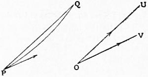
Fig. 64.

§ 13. General Motion of a Particle.—Let P, Q be the positions of a moving point at times t, t + δt respectively. A vector OU> drawn parallel to PQ, of length proportional to PQ/δt on any convenient scale, will represent the mean velocity in the interval δt, i.e. a point moving with a constant velocity having the magnitude and direction indicated by this vector would experience the same resultant displacement PQ> in the same time. As δt is indefinitely diminished, the vector OU> will tend to a definite limit OV>; this is adopted as the definition of the velocity of the moving point at the instant t. Obviously OV> is parallel to the tangent to the path at P, and its magnitude is ds/dt, where s is the arc. If we project OV> on the co-ordinate axes (rectangular or oblique) in the usual manner, the projections u, v, w are called the component velocities parallel to the axes. If x, y, z be the co-ordinates of P it is easily proved that

u = dx , v = dy , w = dz .