VOLUME XIV SLICE V Indole to Insanity (continued 5)

31. Defective modes of expression did not hinder constructive work. It was the great merit of Leibnitz’s symbolism that a mathematician who used it knew what was to be done in order to formulate any problem analytically, Arithmetical basis of modern analysis. even though he might not be absolutely clear as to the proper interpretation of the symbols, or able to render a satisfactory account of them. While new and varied results were promptly obtained by using them, a long time elapsed before the theory of them was placed on a sound basis. Even after Cauchy had formulated his theory much remained to be done, both in the rapidly growing department of complex variables, and in the regions opened up by the theory of expansions in trigonometric series. In both directions it was seen that rigorous demonstration demanded greater precision in regard to fundamental notions, and the requirement of precision led to a gradual shifting of the basis of analysis from geometrical intuition to arithmetical law. A sketch of the outcome of this movement—the “arithmetization of analysis,” as it has been called—will be found in Function. Its general tendency has been to show that many theories and processes, at first accepted as of general validity, are liable to exceptions, and much of the work of the analysts of the latter half of the 19th century was directed to discovering the most general conditions in which particular processes, frequently but not universally applicable, can be used without scruple.

III. Outlines of the Infinitesimal Calculus.

32. The general notions of functionality, limits and continuity are explained in the article Function. Illustrations of the more immediate ways in which these notions present themselves in the development of the differential and integral calculus will be useful in what follows.

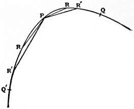
Fig. 8.

33. Let y be given as a function of x, or, more generally, let x and y be given as functions of a variable t. The first of these cases is included in the second by putting x = t. If certain conditions are satisfied the aggregate of the points determined Geometrical limits. by the functional relations form a curve. The first condition is that the aggregate of the values of t to which values of x and y correspond must be continuous, or, in other words, that these values must consist of all real numbers, or of all those real numbers which lie between assigned extreme numbers. When this condition is satisfied the points are “ordered,” and their order is determined by the order of the numbers t, supposed to be arranged in order of increasing or decreasing magnitude; also there are two senses of description of the curve, according as t is taken to increase or to diminish. The second condition is that the aggregate of the points which are determined by the functional relations must be “continuous.” This condition means that, if any point P determined by a value of t is taken, and any distance δ, however small, is chosen, it is possible to find two points Q, Q′ of the aggregate which are such that (i.) P is between Q and Q′, (ii.) if R, R′ are any points between Q and Q′ the distance RR′ is less than δ. The meaning of the word “between” in this statement is fixed by the ordering of the points. Sometimes additional conditions are imposed upon the functional relations before they are regarded as defining a curve. An aggregate of points which satisfies the two conditions stated above is sometimes called a “Jordan curve.” It by no means follows that every curve of this kind has a tangent. In order that the curve Tangents. may have a tangent at P it is necessary that, if any angle α, however small, is specified, a distance δ can be found such that when P is between Q and Q′, and PQ and PQ′ are less than δ, the angle RPR′ is less than α for all pairs of points R, R′ which are between P and Q, or between P and Q′ (fig. 8). When this condition is satisfied y is a function of x which has a differential coefficient. The only way of finding out whether this condition is satisfied or not is to attempt to form the differential coefficient. If the quotient of differences Δy/Δx has a limit when Δx tends to zero, y is a differentiable function of x, and the limit in question is the differential coefficient. The derived function, or differential coefficient, of a function ƒ(x) is always defined by the formula

ƒ′(x) = dƒ(x) = lim.h=0 ƒ(x + h) − ƒ(x) .

dx h

Rules for the formation of differential coefficients in particular cases have been given in § 11 above. The definition of a differential coefficient, and the rules of differentiation are quite independent of any geometrical interpretation, such as that concerning tangents to a curve, and the tangent to a curve is properly defined by means of the differential coefficient of a function, not the differential coefficient by means of the tangent.

It may happen that the limit employed in defining the differential coefficient has one value when h approaches zero through positive values, and a different value when h approaches zero Progressive and Regressive Differential Coefficients. through negative values. The two limits are then called the “progressive” and “regressive” differential coefficients. In applications to dynamics, when x denotes a coordinate and t the time, dx/dt denotes a velocity. If the velocity is changed suddenly the progressive differential coefficient measures the velocity just after the change, and the regressive differential coefficient measures the velocity just before the change. Variable velocities are properly defined by means of differential coefficients.

All geometrical limits may be specified in terms similar to those employed in specifying the tangent to a curve; in difficult cases they must be so specified. Geometrical intuition may fail to answer the question of the existence or non-existence Areas. of the appropriate limits. In the last resort the definitions of many quantities of geometrical import must be analytical, not geometrical. As illustrations of this statement we may take the definitions of the areas and lengths of curves. We may not assume that every curve has an area or a length. To find out whether a curve has an area or not, we must ascertain whether the limit expressed by ƒydx exists. When the limit exists the curve has an area. The definition of the integral is quite independent of any geometrical interpretation. The length of a curve again is defined by means of a limiting process. Let P, Q be two points of a curve, and R1, R2, ... Rn−1 a set of intermediate points of the curve, supposed to be described in the sense in which Q comes after P. The points R are supposed to be reached successively in the order of the suffixes when the curve is described in this sense. We form a sum of lengths of chords

PR1 + R1R2 + ... + Rn−1Q.

If this sum has a limit when the number of the points R is increased indefinitely and the lengths of all the chords are diminished indefinitely, this limit is the length of the arc PQ. The limit Lengths of Curves. is the same whatever law may be adopted for inserting the intermediate points R and diminishing the lengths of the chords. It appears from this statement that the differential element of the arc of a curve is the length of the chord joining two neighbouring points. In accordance with the fundamental artifice for forming differentials (§§ 9, 10), the differential element of arc ds may be expressed by the formula

ds = √ { (dx)2 + (dy)2 },

of which the right-hand member is really the measure of the distance between two neighbouring points on the tangent. The square root must be taken to be positive. We may describe this differential element as being so much of the actual arc between two neighbouring points as need be retained for the purpose of forming the integral expression for an arc. This is a description, not a definition, because the length of the short arc itself is only definable by means of the integral expression. Similar considerations to those used in defining the areas of plane figures and the lengths of plane curves are applicable to the formation of expressions for differential elements of volume or of the areas of curved surfaces.

34. In regard to differential coefficients it is an important theorem Constants of Integration. that, if the derived function ƒ′(x) vanishes at all points of an interval, the function ƒ(x) is constant in the interval. It follows that, if two functions have the same derived function they can only differ by a constant. Conversely, indefinite integrals are indeterminate to the extent of an additive constant.

35. The differential coefficient dy/dx, or the derived function ƒ′(x), is itself a function of x, and its differential coefficient is denoted Higher Differential Coefficients. by ƒ″(x) or d2y/dx2. In the second of these notations d/dx is regarded as the symbol of an operation, that of differentiation with respect to x, and the index 2 means that the operation is repeated. In like manner we may express the results of n successive differentiations by ƒ(n)(x) or by dny/dxn. When the second differential coefficient exists, or the first is differentiable, we have the relation

ƒ″(x) = lim.h=0 ƒ(x + h) − 2ƒ(x) + ƒ(x − h) .

h2

(i.)

The limit expressed by the right-hand member of this equation may exist in cases in which ƒ′(x) does not exist or is not differentiable. The result that, when the limit here expressed can be shown to vanish at all points of an interval, then ƒ(x) must be a linear function of x in the interval, is important.

The relation (i.) is a particular case of the more general relation

ƒ(n)(x) = lim.h=0 h−n [ ƒ(x + nh) − nf {(x + (n − 1) h }

+ n (n − 1) ƒ {x + (n − 2) h } − ... + (−1)n ƒ(x) ].

2!

(ii.)

As in the case of relation (i.) the limit expressed by the right-hand member may exist although some or all of the derived functions ƒ′(x), ƒ″(x), ... ƒ(n−1)(x) do not exist.

Corresponding to the rule iii. of § 11 we have the rule for forming the nth differential coefficient of a product in the form

dn(uv) = u dnv + n du dn−1v + n(n − 1) d2u dn−2v + ... + dnu v,

dxn dxn dx dxn−1 1·2 dx2 dxn−2 dxn

where the coefficients are those of the expansion of (1 + x)n in powers of x (n being a positive integer). The rule is due to Leibnitz, (1695).

Differentials of higher orders may be introduced in the same way as the differential of the first order. In general when y = ƒ(x), the nth differential dny is defined by the equation

dny = ƒ(n) (x) (dx)n,

in which dx is the (arbitrary) differential of x.

When d/dx is regarded as a single symbol of operation the symbol ƒ ... dx represents the inverse operation. If the former is denoted by D, the latter may be denoted by D−1. Dn means that Symbols of operation. the operation D is to be performed n times in succession; D−n that the operation of forming the indefinite integral is to be performed n times in succession. Leibnitz’s course of thought (§ 24) naturally led him to inquire after an interpretation of Dn. where n is not an integer. For an account of the researches to which this inquiry gave rise, reference may be made to the article by A. Voss in Ency. d. math. Wiss. Bd. ii. A, 2 (Leipzig, 1889). The matter is referred to as “fractional” or “generalized” differentiation.

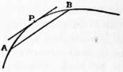
Fig. 9.

36. After the formation of differential coefficients the most important theorem of the differential calculus is the theorem of intermediate value Theorem of Intermediate Value. (“theorem of mean value,” “theorem of finite increments,” “Rolle’s theorem,” are other names for it). This theorem may be explained as follows: Let A, B be two points of a curve y = ƒ(x) (fig. 9). Then there is a point P between A and B at which the tangent is parallel to the secant AB. This theorem is expressed analytically in the statement that if ƒ′(x) is continuous between a and b, there is a value x1 of x between a and b which has the property expressed by the equation

ƒ(b) − ƒ(a) = ƒ′(x1).

b − a

(i.)

The value x1 can be expressed in the form a + θ(b − a) where θ is a number between 0 and 1.

A slightly more general theorem was given by Cauchy (1823) to the effect that, if ƒ′(x) and F′(x) are continuous between x = a and x = b, then there is a number θ between 0 and 1 which has the property expressed by the equation

F(b) − F(a) = F′ {a + θ(b − a) } .

ƒ(b) − ƒ(a) ƒ′ {a + θ(b − a) }

The theorem expressed by the relation (i.) was first noted by Rolle (1690) for the case where ƒ(x) is a rational integral function which vanishes when x = a and also when x = b. The general theorem was given by Lagrange (1797). Its fundamental importance was first recognized by Cauchy (1823). It may be observed here that the theorem of integral calculus expressed by the equation

F(b) − F(a) = ∫ba F′(x) dx

follows at once from the definition of an integral and the theorem of intermediate value.

The theorem of intermediate value may be generalized in the statement that, if ƒ(x) and all its differential coefficients up to the nth inclusive are continuous in the interval between x = a and x = b, then there is a number θ between 0 and 1 which has the property expressed by the equation

ƒ(b) = ƒ(a) + (b − a) ƒ′(a) + (b − a)2 ƒ″(a) + ... + (b − a)n−1 ƒ(n−1)(a)

2! (n − 1)!

+ (b − a)n ƒ(n) {a + θ (b − a) }.

n!

(ii.)

37. This theorem provides a means for computing the values of a function at points near to an assigned point when the value of the function and its differential coefficients at the assigned point are known. The function is expressed by a terminated Taylor’s Theorem. series, and, when the remainder tends to zero as n increases, it may be transformed into an infinite series. The theorem was first given by Brook Taylor in his Methodus Incrementorum (1717) as a corollary to a theorem concerning finite differences. Taylor gave the expression for ƒ(x + z) in terms of ƒ(x), ƒ′(x), ... as an infinite series proceeding by powers of z. His notation was that appropriate to the method of fluxions which he used. This rule for expressing a function as an infinite series is known as Taylor’s theorem. The relation (i.), in which the remainder after n terms is put in evidence, was first obtained by Lagrange (1797). Another form of the remainder was given by Cauchy (1823) viz.,

(b − a)n (1 − θ)n−1 ƒn {a + θ(b − a) }.

(n − 1)!

The conditions of validity of Taylor’s expansion in an infinite series have been investigated very completely by A. Pringsheim (Math. Ann. Bd. xliv., 1894). It is not sufficient that the function and all its differential coefficients should be finite at x = a; there must be a neighbourhood of a within which Cauchy’s form of the remainder tends to zero as n increases (cf. Function).

An example of the necessity of this condition is afforded by the function f(x) which is given by the equation

ƒ(x) = 1 + Σn=∞n=1 (−1)n 1 .

1 + x2 n! 1 + 32n x2

(i.)

The sum of the series

ƒ(0) + xƒ′(0) + x2 ƒ″(0)+ ...

2!

(ii.)

is the same as that of the series

e−1 − x2 e−32 + x4 e−34 − ...

It is easy to prove that this is less than e−1 when x lies between 0 and 1, and also that f(x) is greater than e−l when x = 1/√3. Hence the sum of the series (i.) is not equal to the sum of the series (ii.).

The particular case of Taylor’s theorem in which a = 0 is often called Maclaurin’s theorem, because it was first explicitly stated by Colin Maclaurin in his Treatise of Fluxions (1742). Maclaurin like Taylor worked exclusively with the fluxional calculus.

Examples of expansions in series had been known for some time. The series for log (1 + x) was obtained by Nicolaus Mercator (1668) by expanding (1 + x)−1 by the method of algebraic division, and integrating the series term by term. He Expansions in power series. regarded his result as a “quadrature of the hyperbola.” Newton (1669) obtained the expansion of sin−1x by expanding (l − x2)−1/2 by the binomial theorem and integrating the series term by term. James Gregory (1671) gave the series for tan−1x. Newton also obtained the series for sin x, cos x, and ex by reversion of series (1669). The symbol e for the base of the Napierian logarithms was introduced by Euler (1739). All these series can be obtained at once by Taylor’s theorem. James Gregory found also the first few terms of the series for tan x and sec x; the terms of these series may be found successively by Taylor’s theorem, but the numerical coefficient of the general term cannot be obtained in this way.

Taylor’s theorem for the expansion of a function in a power series was the basis of Lagrange’s theory of functions, and it is fundamental also in the theory of analytic functions of a complex variable as developed later by Karl Weierstrass. It has also numerous applications to problems of maxima and minima and to analytical geometry. These matters are treated in the appropriate articles.

The forms of the coefficients in the series for tan x and sec x can be expressed most simply in terms of a set of numbers introduced by James Bernoulli in his treatise on probability entitled Ars Conjectandi (1713). These numbers B1, B2, ... called Bernoulli’s numbers, are the coefficients so denoted in the formula

x = 1 − x + B1 x2 − B2 x4 + B3 x6 − ...,

ex − 1 2 2! 4! 6!

and they are connected with the sums of powers of the reciprocals of the natural numbers by equations of the type

Bn = (2n)! ( 1 + 1 + 1 + ... ).

22n−1 π2n 12n 22n 32n

The function

xm − m xm−1 + m·m − 1 B1 xm−2 − ...

2 2!

has been called Bernoulli’s function of the mth order by J. L. Raabe (Crelle’s J. f. Math. Bd. xlii., 1851). Bernoulli’s numbers and functions are of especial importance in the calculus of finite differences (see the article by D. Seliwanoff in Ency. d. math. Wiss. Bd. i., E., 1901).

When x is given in terms of y by means of a power series of the form

x = y (C0 + C1y + C2y2 + ...) (C0 ≠ 0) = yƒ0(y), say,

there arises the problem of expressing y as a power series in x. This problem is that of reversion of series. It can be shown that provided the absolute value of x is not too great,

y = x + Σn=∞n=2 [ xn · dn−1 1 ]y=0

ƒ0(0) n! dyn−1 {ƒ0(y)}n

To this problem is reducible that of expanding y in powers of x when x and y are connected by an equation of the form

y = a + xƒ(y),

for which problem Lagrange (1770) obtained the formula

y = a + xƒ(a) + Σn=∞n=2 [ n · dn−1 {ƒ(a)}n ].

n! dan−1

For the history of the problem and the generalizations of Lagrange’s result reference may be made to O. Stolz, Grundzüge d. Diff. u. Int. Rechnung, T. 2 (Leipzig, 1896).

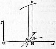
Fig. 10.

38. An important application of the theorem of intermediate value and its generalization can be made to the problem of evaluating certain limits. If two functions φ(x) and ψ(x) both vanish at x = a, the fraction φ(x)/ψ(x) may have a finite Indeterminate forms. limit at a. This limit is described as the limit of an “indeterminate form.” Such indeterminate forms were considered first by de l’Hospital (1696) to whom the problem of evaluating the limit presented itself in the form of tracing the curve y = φ(x)/ψ(x) near the ordinate x = a, when the curves y = φ(x) and y = ψ(x) both cross the axis of x at the same point as this ordinate. In fig. 10 PA and QA represent short arcs of the curves φ, ψ, chosen so that P and Q have the same abscissa. The value of the ordinate of the corresponding point R of the compound curve is given by the ratio of the ordinates PM, QM. De l’Hospital treated PM and QM as “infinitesimal,” so that the equations PM : AM =φ’(a) and QM : AM = ψ′(a) could be assumed to hold, and he arrived at the result that the “true value” of φ(a)/ψ(a) is φ′(a)/ψ′(a). It can be proved rigorously that, if ψ′(x) does not vanish at x = a, while φ(a) = 0 and ψ(a) = 0, then

lim.x=a φ(x) = φ′(a) .

ψ(x) ψ′(a)

It can be proved further if that φm(x) and ψn(x) are the differential coefficients of lowest order of φ(x) and ψ(x) which do not vanish at x = a, and if m = n, then

lim.x=a φ(x) = φn(a) .

ψ(x) ψn(a)

If m > n the limit is zero; but if m < n the function represented by the quotient φ(x)/ψ(x) “becomes infinite” at x = a. If the value of the function at x = a is not assigned by the definition of the function, the function does not exist at x = a, and the meaning of the statement that it “becomes infinite” is that it has no finite limit. The statement does not mean that the function has a value which we call infinity. There is no such value (see Function).

Such indeterminate forms as that described above are said to be of the form 0/0. Other indeterminate forms are presented in the form 0 × ∞, or 1∞, or ∞/∞, or ∞ − ∞. The most notable of the forms 1∞ is lim.x=0(1 + x)1/x, which is e. The case in which φ(x) and ψ(x) both tend to become infinite at x = a is reducible to the case in which both the functions tend to become infinite when x is increased indefinitely. If φ′(x) and ψ′(x) have determinate finite limits when x is increased indefinitely, while φ(x) and ψ(x) are determinately (positively or negatively) infinite, we have the result expressed by the equation

lim.x=∞ φ(x) = lim.x=∞ φ′(x) .

ψ(x) lim.x=∞ ψ′(x)

For the meaning of the statement that φ(x) and ψ(x) are determinately infinite reference may be made to the article Function. The evaluation of forms of the type ∞/∞ leads to a scale of increasing “infinities,” each being infinite in comparison with the preceding. Such a scale is

log x, ... x, x2, ... xn, ... ex, ... xx;

each of the limits expressed by such forms as lim.x=∞ φ(x)/ψ(x), where φ(x) precedes ψ(x) in the scale, is zero. The construction of such scales, along with the problem of constructing a complete scale was discussed in numerous writings by Paul du Bois-Reymond (see in particular, Math. Ann. Bd. xi., 1877). For the general problem of indeterminate forms reference may be made to the article by A. Pringsheim in Ency. d. math. Wiss. Bd. ii., A. 1 (1899). Forms of the type 0/0 presented themselves to early writers on analytical geometry in connexion with the determination of the tangents at a double point of a curve; forms of the type ∞/∞ presented themselves in like manner in connexion with the determination of asymptotes of curves. The evaluation of limits has innumerable applications in all parts of analysis. Cauchy’s Analyse algébrique (1821) was an epoch-making treatise on limits.

If a function φ(x) becomes infinite at x = a, and another function ψ(x) also becomes infinite at x = a in such a way that φ(x)/ψ(x) has a finite limit C, we say that φ(x) and ψ(x) become “infinite of the same order.” We may write φ(x) = Cψ(x) + φ1(x), where lim.x=aφ1(x)/ψ(x) = 0, and thus φ1(x) is of a lower order than φ(x); it may be finite or infinite at x = a. If it is finite, we describe Cψ(x) as the “infinite part” of φ(x). The resolution of a function which becomes infinite into an infinite part and a finite part can often be effected by taking the infinite part to be infinite of the same order as one of the functions in the scale written above, or in some more comprehensive scale. This resolution is the inverse of the process of evaluating an indeterminate form of the type ∞ − ∞.

For example lim.x=0{(ex − 1)−1 − x−1} is finite and equal to = ½, and the function (ex − 1)−1 − x−1 can be expanded in a power series in x.

39. Functions of several variables. The nature of a function of two or more variables, and the meaning to be attached to continuity and limits in respect of such functions, have been explained under Function. The theorems of differential calculus which relate to such functions are in general the same whether the number of variables is two or any greater number, and it will generally be convenient to state the theorems for two variables.

40. Let u or ƒ (x, y) denote a function of two variables x and y. If we regard y as constant, u or ƒ becomes a function of one variable x, and we may seek to differentiate it with respect to x. If the function of x is differentiable, the differential Partial differentiation. coefficient which is formed in this way is called the “partial differential coefficient” of u or ƒ with respect to x, and is denoted by ∂u/∂x or ∂ƒ/∂x. The symbol “∂” was appropriated for partial differentiation by C. G. J. Jacobi (1841). It had before been written indifferently with “d” as a symbol of differentiation. Euler had written (dƒ/dx) for the partial differential coefficient of ƒ with respect to x. Sometimes it is desirable to put in evidence the variable which is treated as constant, and then the partial differential coefficient is written “(dƒ/dx)y” or “(∂ƒ/∂x)y”. This course is often adopted by writers on Thermodynamics. Sometimes the symbols d or ∂ are dropped, and the partial differential coefficient is denoted by ux or ƒx. As a definition of the partial differential coefficient we have the formula

∂ƒ = lim.h=0 ƒ(x + h, y) − ƒ(x, y) .

∂x h

In the same way we may form the partial differential coefficient with respect to y by treating x as a constant.

The introduction of partial differential coefficients enables us to solve at once for a surface a problem analogous to the problem of tangents for a curve; and it also enables us to take the first step in the solution of the problem of maxima and minima for a function of several variables. If the equation of a surface is expressed in the form z = ƒ(x, y), the direction cosines of the normal to the surface at any point are in the ratios ∂ƒ/∂x : ∂ƒ/∂y : = 1. If f is a maximum or a minimum at (x, y), then ∂ƒ/∂x and ∂ƒ/∂y vanish at that point.

In applications of the differential calculus to mathematical physics we are in general concerned with functions of three variables x, y, z, which represent the coordinates of a point; and then considerable importance attaches to partial differential coefficients which are formed by a particular rule. Let F(x, y, z) be the function, P a point (x, y, z), P′ a neighbouring point (x + Δx, y + Δy, z + Δz), and let Δs be the length of PP′. The value of F(x, y, z) at P may be denoted shortly by F(P). A limit of the same nature as a partial differential coefficient is expressed by the formula

lim.Δs=0 F(P′) = F(P) ,

Δs

in which Δs is diminished indefinitely by bringing P′ up to P, and P′ is supposed to approach P along a straight line, for example, the tangent to a curve or the normal to a surface. The limit in question is denoted by ∂F/∂h, in which it is understood that h indicates a direction, that of PP′. If l, m, n are the direction cosines of the limiting direction of the line PP′, supposed drawn from P to P′, then

∂F ∂F ∂F ∂F .

∂h ∂x ∂y ∂z

The operation of forming ∂F/∂h is called “differentiation with respect to an axis” or “vector differentiation.”

41. The most important theorem in regard to partial differential coefficients is the theorem of the total differential. We may write down the equation

ƒ(a + h, b + k) − ƒ(a, b) = ƒ(a + h, b + k) − ƒ(a, b + k) + ƒ(a, b + k) − ƒ(a, b).

If Theorem of the Total Differential. ƒx is a continuous function of x when x lies between a and a + h and y = b + k, and if further ƒy is a continuous function of y when y lies between b and d + k, there exist values of θ and η which lie between 0 and 1 and have the properties expressed by the equations

ƒ(a + h, b + k) − ƒ(a, b + k) = hƒx(a + θh, b + k), ƒ(a, b + k) − ƒ(a, b) = kƒy(a, b + ηk).

Further, ƒx(a + θh, b + k) and ƒy(a, b + ηk) tend to the limits ƒx(a, b) and ƒy(a, b) when h and k tend to zero, provided the differential coefficients ƒx, ƒy, are continuous at the point (a, b). Hence in this case the above equation can be written

ƒ(a + h, b + k) − ƒ(a, b) = hƒx(a, b) + kƒy(a, b) + R,

where

lim.h=0, k=0 R = 0 and lim.h=0, k=0 R = 0.

h k

In accordance with the notation of differentials this equation gives

dƒ = ∂f dx + ∂y dy.

∂x ∂y

Just as in the case of functions of one variable, dx and dy are arbitrary finite differences, and dƒ is not the difference of two values of ƒ, but is so much of this difference as need be retained for the purpose of forming differential coefficients.

The theorem of the total differential is immediately applicable to the differentiation of implicit functions. When y is a function of x which is given by an equation of the form ƒ(x, y) = 0, and it is either impossible or inconvenient to solve this equation so as to express y as an explicit function of x, the differential coefficient dy/dx can be formed without solving the equation. We have at once

dy = − ∂ƒ / ∂ƒ .

dx ∂x ∂y

This rule was known, in all essentials, to Fermat and de Sluse before the invention of the algorithm, of the differential calculus.

An important theorem, first proved by Euler, is immediately deducible from the theorem of the total differential. If ƒ(x, y) is a homogeneous function of degree n then

x ∂f + y ∂f = nƒ(x, y).

∂x ∂y

The theorem is applicable to functions of any number of variables and is generally known as Euler’s theorem of homogeneous functions.

42. Jacobians.Many problems in which partial differential coefficients occur are simplified by the introduction of certain determinants called “Jacobians” or “functional determinants.” They were introduced into Analysis by C. G. J. Jacobi (J. f. Math., Crelle, Bd. 22, 1841, p. 319). The Jacobian of u1, u2, ... un with respect to x1, x2, ... xn is the determinant

∂u1 ∂u1 ... ∂u1 ∂x1 ∂x2 ∂xn

∂u2 ∂u2 ... ∂u2 ∂x1 ∂x2 ∂xn

:

∂un ∂un ... ∂un ∂x1 ∂x2 ∂xn

in which the constituents of the rth row are the n partial differential coefficients of ur, with respect to the n variables x. This determinant is expressed shortly by

∂(u1, u2, ..., un) .

∂(x1, x2, ..., xn)

Jacobians possess many properties analogous to those of ordinary differential coefficients, for example, the following:—

∂(u1, u2, ..., un) × ∂(x1, x2, ..., xn) = 1,

∂(x1, x2, ..., xn) ∂(u1, u2, ..., un)

∂(u1, u2, ..., un) × ∂(y1, y2, ..., yn) = ∂(u1, u2, ..., un) .

∂(y1, y2, ..., yn) ∂(x1, x2, ..., xn) ∂(x1, x2, ..., xn)

If n functions (u1, u2, ... un) of n variables (x1, x2, ..., xn) are not independent, but are connected by a relation ƒ(u1, u2, ... un) = 0, then

∂(u1, u2, ..., un) = 0;

∂(x1, x2, ..., xn)

and, conversely, when this condition is satisfied identically the functions u1, u2 ..., un are not independent.

43. Partial differential coefficients of the second and higher Interchange of order of differentiations. orders can be formed in the same way as those of the first order. For example, when there are two variables x, y, the first partial derivatives ∂ƒ/∂x and ∂ƒ/∂y are functions of x and y, which we may seek to differentiate partially with respect to x or y. The most important theorem in relation to partial differential coefficients of orders higher than the first is the theorem that the values of such coefficients do not depend upon the order in which the differentiations are performed. For example, we have the equation

∂ ( ∂ƒ ) = ∂ ( ∂ƒ ).

∂x ∂y ∂y ∂x

(i.)

This theorem is not true without limitation. The conditions for its validity have been investigated very completely by H. A. Schwarz (see his Ges. math. Abhandlungen, Bd. 2, Berlin, 1890, p. 275). It is a sufficient, though not a necessary, condition that all the differential coefficients concerned should be continuous functions of x, y. In consequence of the relation (i.) the differential coefficients expressed in the two members of this relation are written

∂2ƒ or ∂2ƒ .

∂x∂y ∂y∂x

The differential coefficient

∂nƒ ,

∂xp ∂yq ∂zr

in which p + g + r = n, is formed by differentiating p times with respect to x, q times with respect to y, r times with respect to z, the differentiations being performed in any order. Abbreviated notations are sometimes used in such forms as

ƒ xp yq zr or ƒ (p, q, r) .

x, y, z

Differentials of higher orders are introduced by the defining equation

dnƒ = ( dx ∂ + dy ∂ ) n ƒ

∂x ∂y

= (dx)n ∂nƒ + n(dx)n−1 dy ∂nƒ + ...

∂xn ∂xn−1 ∂y

in which the expression (dx·∂/∂x + dy·∂/∂y)n is developed by the binomial theorem in the same way as if dx·∂/∂x and dy·∂/∂y were numbers, and (∂/∂x)r·(∂/∂y)n−r ƒ is replaced by ∂nƒ/∂xr ∂yn−r. When there are more than two variables the multinomial theorem must be used instead of the binomial theorem.

The problem of forming the second and higher differential coefficients of implicit functions can be solved at once by means of partial differential coefficients, for example, if ƒ(x, y) = 0 is the equation defining y as a function of x, we have

d2y = ( ∂ƒ ) −3 { ( ∂ƒ )2 ∂2ƒ − 2 ∂ƒ · ∂ƒ · ∂2ƒ + ( ∂ƒ )2 ∂2ƒ }.

dx2 ∂y ∂y ∂x2 ∂x ∂y ∂x∂y ∂x ∂y2

The differential expression Xdx + Ydy, in which both X and Y are functions of the two variables x and y, is a total differential if there exists a function ƒ of x and y which is such that

∂ƒ/∂x = X, ∂ƒ/∂y = Y.

When this is the case we have the relation

∂Y/∂x = ∂X/∂y.

(ii.)

Conversely, when this equation is satisfied there exists a function ƒ which is such that

dƒ= Xdx + Ydy.

The expression Xdx + Ydy in which X and Y are connected by the relation (ii.) is often described as a “perfect differential.” The theory of the perfect differential can be extended to functions of n variables, and in this case there are ½n(n − 1) such relations as (ii.).

In the case of a function of two variables x, y an abbreviated notation is often adopted for differential coefficients. The function being denoted by z, we write

p, q, r, s, t for ∂z , ∂z , ∂2z , ∂2z , ∂2z .

∂x ∂y ∂x2 ∂x∂y ∂y2

Partial differential coefficients of the second order are important in geometry as expressing the curvature of surfaces. When a surface is given by an equation of the form z = ƒ(x, y), the lines of curvature are determined by the equation

{ (l + q2)s − pqt} (dy)2 + { (1 + q2)r − (1 + p2)t } dxdy − { (1 + p2)s − pqr} (dx)2 = 0,

and the principal radii of curvature are the values of R which satisfy the equation

R2(rt − s2) − R { (1 + q2)r − 2pqs + (1 + p2)t } √(1 + p2 + q2) + (1 + p2 + q2)2 = 0.

44. Change of variables.The problem of change of variables was first considered by Brook Taylor in his Methodus incrementorum. In the case considered by Taylor y is expressed as a function of z, and z as a function of x, and it is desired to express the differential coefficients of y with respect to x without eliminating z. The result can be obtained at once by the rules for differentiating a product and a function of a function. We have

dy = dy · dz ,

dx dz dx

d2y = dy · d2z + d2y · ( dz )2,

dx2 dz dx2 dz2 dx

d3y = dy · d3z + 3 d2y · dz · d2z + d3y · ( dz )3,

dx3 dz dx3 dz2 dx dx2 dz3 dx

. . . . . . . . . . . . . . . . . . . . .

The introduction of partial differential coefficients enables us to deal with more general cases of change of variables than that considered above. If u, v are new variables, and x, y are connected with them by equations of the type

x = ƒ1(u, v), y = ƒ2(u, v),

(i.)

while y is either an explicit or an implicit function of x, we have the problem of expressing the differential coefficients of various orders of y with respect to x in terms of the differential coefficients of v with respect to u. We have

dy = ( ∂ƒ2 + ∂ƒ2 dv ) / ( ∂ƒ1 + ∂ƒ1 dv )

dx ∂u ∂v du ∂u ∂v du

by the rule of the total differential. In the same way, by means of differentials of higher orders, we may express d2y/dx2, and so on.

Equations such as (i.) may be interpreted as effecting a transformation by which a point (u, v) is made to correspond to a point (x, y). The whole theory of transformations, and of functions, or differential expressions, which remain invariant under groups of transformations, has been studied exhaustively by Sophus Lie (see, in particular, his Theorie der Transformationsgruppen, Leipzig, 1888-1893). (See also Differential Equations and Groups).

A more general problem of change of variables is presented when it is desired to express the partial differential coefficients of a function V with respect to x, y, ... in terms of those with respect to u, v, ..., where u, v, ... are connected with x, y, ... by any functional relations. When there are two variables x, y, and u, v are given functions of x, y, we have

∂V = ∂V ∂u + ∂V ∂v ,

∂x ∂u ∂x ∂v ∂x

∂V = ∂V ∂u + ∂V ∂v ,

∂y ∂u ∂y ∂v ∂y

and the differential coefficients of higher orders are to be formed by repeated applications of the rule for differentiating a product and the rules of the type

∂ = ∂u ∂ + ∂v ∂ .

∂x ∂x ∂u ∂x ∂v

When x, y are given functions of u, v, ... we have, instead of the above, such equations as

∂V = ∂V ∂x + ∂V ∂y ;

∂u ∂x ∂u ∂y ∂u

and ∂V/∂x, ∂V/∂y can be found by solving these equations, provided the Jacobian ∂(x, y)/∂(u, v) is not zero. The generalization of this method for the case of more than two variables need not detain us.

In cases like that here considered it is sometimes more convenient not to regard the equations connecting x, y with u, v as effecting a point transformation, but to consider the loci u = const., v = const. as two “families” of curves. Then in any region of the plane of (x, y) in which the Jacobian ∂(x, y)/∂(u, v) does not vanish or become infinite, any point (x, y) is uniquely determined by the values of u and v which belong to the curves of the two families that pass through the point. Such variables as u, v are then described as “curvilinear coordinates” of the point. This method is applicable to any number of variables. When the loci u = const., ... intersect each other at right angles, the variables are “orthogonal” curvilinear coordinates. Three-dimensional systems of such coordinates have important applications in mathematical physics. Reference may be made to G. Lamé, Leçons sur les coordonnées curvilignes (Paris, 1859), and to G. Darboux, Leçons sur les coordonnées curvilignes et systèmes orthogonaux (Paris, 1898).

When such a coordinate as u is connected with x and y by a functional relation of the form ƒ(x, y, u) = 0 the curves u = const. are a family of curves, and this family may be such that no two curves of the family have a common point. When this is not the case the points in which a curve ƒ(x, y, u) = 0 is intersected by a curve ƒ(x, y, u + Δu) = 0 tend to limiting positions as Δu is diminished indefinitely. The locus of these limiting positions is the “envelope” of the family, and in general it touches all the curves of the family. It is easy to see that, if u, v are the parameters of two families of curves which have envelopes, the Jacobian ∂(x, y)/∂(u, v) vanishes at all points on these envelopes. It is easy to see also that at any point where the reciprocal Jacobian ∂(u, v)/∂(x, y) vanishes, a curve of the family u touches a curve of the family v.

If three variables x, y, z are connected by a functional relation ƒ(x, y, z) = 0, one of them, z say, may be regarded as an implicit function of the other two, and the partial differential coefficients of z with respect to x and y can be formed by the rule of the total differential. We have

∂z = − ∂ƒ / ∂ƒ , ∂z = − ∂ƒ / ∂ƒ ;

∂x ∂x ∂z ∂y ∂y ∂z

and there is no difficulty in proceeding to express the higher differential coefficients. There arises the problem of expressing the partial differential coefficients of x with respect to y and z in terms of those of z with respect to x and y. The problem is known as that of “changing the dependent variable.” It is solved by applying the rule of the total differential. Similar considerations are applicable to all cases in which n variables are connected by fewer than n equations.

45. Extension of Taylor’s theorem.Taylor’s theorem can be extended to functions of several variables. In the case of two variables the general formula, with a remainder after n terms, can be written most simply in the form

ƒ(a + h, b + k) = ƒ(a, b) + dƒ(a, b) + 1 d2 ƒ(a, b) + ...

2!

+ 1 dn−1 ƒ(a, b) + 1 dn ƒ(a + θh, b + θk),

(n − 1)! n!

in which

dr ƒ(a, b) = [ ( h ∂ + k ∂ )rƒ(x, y) ] ,

∂x ∂y x=a, y=b

and

dn ƒ(a + θh, b + θk) = [ ( h ∂ + k ∂ )nƒ(x, y) ] .

∂x ∂y x=a+θh, y=b+θk

The last expression is the remainder after n terms, and in it θ denotes some particular number between 0 and 1. The results for three or more variables can be written in the same form. The extension of Taylor’s theorem was given by Lagrange (1797); the form written above is due to Cauchy (1823). For the validity of the theorem in this form it is necessary that all the differential coefficients up to the nth should be continuous in a region bounded by x = a ± h, y = b ± k. When all the differential coefficients, no matter how high the order, are continuous in such a region, the theorem leads to an expansion of the function in a multiple power series. Such expansions are just as important in analysis, geometry and mechanics as expansions of functions of one variable. Among the problems which are solved by means of such expansions are the problem of maxima and minima for functions of more than one variable (see Maxima and Minima).

46. Plane curves.In treatises on the differential calculus much space is usually devoted to the differential geometry of curves and surfaces. A few remarks and results relating to the differential geometry of plane curves are set down here.

(i.) If ψ denotes the angle which the radius vector drawn from the origin makes with the tangent to a curve at a point whose polar coordinates are r, θ and if p denotes the perpendicular from the origin to the tangent, then

cos ψ = dr/ds, sin ψ = rdθ/ds = p/r,

where ds denotes the element of arc. The curve may be determined by an equation connecting p with r.

(ii.) The locus of the foot of the perpendicular let fall from the origin upon the tangent to a curve at a point is called the pedal of the curve with respect to the origin. The angle ψ for the pedal is the same as the angle ψ for the curve. Hence the (p, r) equation of the pedal can be deduced. If the pedal is regarded as the primary curve, the curve of which it is the pedal is the “negative pedal” of the primary. We may have pedals of pedals and so on, also negative pedals of negative pedals and so on. Negative pedals are usually determined as envelopes.

(iii.) If φ denotes the angle which the tangent at any point makes with a fixed line, we have

r2 = p2 + (dp/dφ)2.

(iv.) The “average curvature” of the arc Δs of a curve between two points is measured by the quotient

Δφ Δs

where the upright lines denote, as usual, that the absolute value of the included expression is to be taken, and φ is the angle which the tangent makes with a fixed line, so that Δφ is the angle between the tangents (or normals) at the points. As one of the points moves up to coincidence with the other this average curvature tends to a limit which is the “curvature” of the curve at the point. It is denoted by

dφ ds

Sometimes the upright lines are omitted and a rule of signs is given:—Let the arc s of the curve be measured from some point along the curve in a chosen sense, and let the normal be drawn towards that side to which the curve is concave; if the normal is directed towards the left of an observer looking along the tangent in the chosen sense of description the curvature is reckoned positive, in the contrary case negative. The differential dφ is often called the “angle of contingence.” In the 14th century the size of the angle between a curve and its tangent seems to have been seriously debated, and the name “angle of contingence” was then given to the supposed angle.

(v.) The curvature of a curve at a point is the same as that of a certain circle which touches the curve at the point, and the “radius of curvature” ρ is the radius of this circle. We have 1/ρ = |dφ/ds|. The centre of the circle is called the “centre of curvature”; it is the limiting position of the point of intersection of the normal at the point and the normal at a neighbouring point, when the second point moves up to coincidence with the first. If a circle is described to intersect the curve at the point P and at two other points, and one of these two points is moved up to coincidence with P, the circle touches the curve at the point P and meets it in another point; the centre of the circle is then on the normal. As the third point now moves up to coincidence with P, the centre of the circle moves to the centre of curvature. The circle is then said to “osculate” the curve, or to have “contact of the second order” with it at P.

(vi.) The following are formulae for the radius of curvature:—

1 = | { 1 + ( dy )2 }−3/2 d2y |,

ρ dx dx2

ρ = | r dr | = | p + d2p |.

dp dφ2

(vii.) The points at which the curvature vanishes are “points of inflection.” If P is a point of inflection and Q a neighbouring point, then, as Q moves up to coincidence with P, the distance from P to the point of intersection of the normals at P and Q becomes greater than any distance that can be assigned. The equation which gives the abscissae of the points in which a straight line meets the curve being expressed in the form ƒ(x) = 0, the function ƒ(x) has a factor (x − x0)3, where x0 is the abscissa of the point of inflection P, and the line is the tangent at P. When the factor (x − x0) occurs (n + 1) times in ƒ(x), the curve is said to have “contact of the nth order” with the line. There is an obvious modification when the line is parallel to the axis of y.

(viii.) The locus of the centres of curvature, or envelope of the normals, of a curve is called the “evolute.” A curve which has a given curve as evolute is called an “involute” of the given curve. All the involutes are “parallel” curves, that is to say, they are such that one is derived from another by marking off a constant distance along the normal. The involutes are “orthogonal trajectories” of the tangents to the common evolute.

(ix.) The equation of an algebraic curve of the nth degree can be expressed in the form u0 + u1 + u2 + ... + un = 0, where u0 is a constant, and ur is a homogeneous rational integral function of x, y of the rth degree. When the origin is on the curve, u0 vanishes, and u1 = 0 represents the tangent at the origin. If u1 also vanishes, the origin is a double point and u2 = o represents the tangents at the origin. If u2 has distinct factors, or is of the form a(y − p1x) (y − p2x), the value of y on either branch of the curve can be expressed (for points sufficiently near the origin) in a power series, which is either

p1x + ½ q1 x2 + ..., or p2x + ½ q2 x2 + ...,

where q1, ... and q2, ... are determined without ambiguity. If p1 and p2 are real the two branches have radii of curvature ρ1, ρ2 determined by the formulae

1 = | (1 + p12)−3/2 q1 |, 1 = | (1 + p22)−3/2 q2 |.

ρ1 ρ2

When p1 and p2 are imaginary the origin is the real point of intersection of two imaginary branches. In the real figure of the curve it is an isolated point. If u2 is a square, a(y − px)2, the origin is a cusp, and in general there is not a series for y in integral powers of x, which is valid in the neighbourhood of the origin. The further investigation of cusps and multiple points belongs rather to analytical geometry and the theory of algebraic functions than to differential calculus.

(x.) When the equation of a curve is given in the form u0 + u1 + ... + un−1 + un = 0 where the notation is the same as that in (ix.), the factors of un determine the directions of the asymptotes. If these factors are all real and distinct, there is an asymptote corresponding to each factor. If un = L1L2 ... Ln, where L1, ... are linear in x, y, we may resolve un−1/un into partial fractions according to the formula

un−1 = A1 + A2 + ... + An ,

un L1 L2 Ln

and then L1 + A1 = 0, L2 + A2 = 0, ... are the equations of the asymptotes. When a real factor of un is repeated we may have two parallel asymptotes or we may have a “parabolic asymptote.” Sometimes the parallel asymptotes coincide, as in the curve x2(x2 + y2 − a2) = a4, where x = 0 is the only real asymptote. The whole theory of asymptotes belongs properly to analytical geometry and the theory of algebraic functions.

47. The formal definition of an integral, the theorem of the existence of the integral for certain classes of functions, a list of Integral calculus. classes of “integrable” functions, extensions of the notion of integration to functions which become infinite or indeterminate, and to cases in which the limits of integration become infinite, the definitions of multiple integrals, and the possibility of defining functions by means of definite integrals—all these matters have been considered in Function. The definition of integration has been explained in § 5 above, and the results of some of the simplest integrations have been given in § 12. A few theorems relating to integrations have been noted in §§ 34, 35, 36 above.

48. Methods of integration.The chief methods for the evaluation of indefinite integrals are the method of integration by parts, and the introduction of new variables.

From the equation d(uv) = u dv + v du we deduce the equation

∫ u dv dx = uv − ∫ v du dx,

dx dx

or, as it may be written

∫ uw dx = u ∫ w dx − ∫ du { ∫ w dx } dx.

dx

This is the rule of “integration by parts.”

As an example we have

∫ xeax dx = x eax − ∫ eax dx = ( x − 1 ) eax.

a a a a2

When we introduce a new variable z in place of x, by means of an equation giving x in terms of z, we express ƒ(x) in terms of z. Let φ(z) denote the function of z into which ƒ(x) is transformed. Then from the equation

dx = dx dz

dz

we deduce the equation

∫ ƒ(x) dx = ∫ φ(z) dx dz.

dz

As an example, in the integral

∫ √(1 − x2)dx

put x = sin z; the integral becomes

∫ cos z · cos z dz = ∫ ½ (1 + cos 2z)dz = ½ (z + ½ sin 2z) = ½ (z + sin z cos z).

49. The indefinite integrals of certain classes of functions can be expressed by means of a finite number of operations of addition or multiplication in terms of the so-called “elementary” functions. The elementary functions are rational algebraic Integration in terms of elementary functions. functions, implicit algebraic functions, exponentials and logarithms, trigonometrical and inverse circular functions. The following are among the classes of functions whose integrals involve the elementary functions only: (i.) all rational functions; (ii.) all irrational functions of the form ƒ(x, y), where ƒ denotes a rational algebraic function of x and y, and y is connected with x by an algebraic equation of the second degree; (iii.) all rational functions of sin x and cos x; (iv.) all rational functions of ex; (v.) all rational integral functions of the variables x, eax, ebx, ... sin mx, cos mx, sin nx, cos nx, ... in which a, b, ... and m, n, ... are any constants. The integration of a rational function is generally effected by resolving the function into partial fractions, the function being first expressed as the quotient of two rational integral functions. Corresponding to any simple root of the denominator there is a logarithmic term in the integral. If any of the roots of the denominator are repeated there are rational algebraic terms in the integral. The operation of resolving a fraction into partial fractions requires a knowledge of the roots of the denominator, but the algebraic part of the integral can always be found without obtaining all the roots of the denominator. Reference may be made to C. Hermite, Cours d’analyse, Paris, 1873. The integration of other functions, which can be integrated in terms of the elementary functions, can usually be effected by transforming the functions into rational functions, possibly after preliminary integrations by parts. In the case of rational functions of x and a radical of the form √(ax2 + bx + c) the radical can be reduced by a linear substitution to one of the forms √(a2 − x2), √(x2 − a2), √(x2 + a2). The substitutions x = a sin θ, x = a sec θ, x = a tan θ are then effective in the three cases. By these substitutions the subject of integration becomes a rational function of sin θ and cos θ, and it can be reduced to a rational function of t by the substitution tan ½θ = t. There are many other substitutions by which such integrals can be determined. Sometimes we may have information as to the functional character of the integral without being able to determine it. For example, when the subject of integration is of the form (ax4 + bx3 + cx2 + dx + e)−1/2 the integral cannot be expressed explicitly in terms of elementary functions. Such integrals lead to new functions (see Function).

Methods of reduction and substitution for the evaluation of indefinite integrals occupy a considerable space in text-books of the integral calculus. In regard to the functional character of the integral reference may be made to G. H. Hardy’s tract, The Integration of Functions of a Single Variable (Cambridge, 1905), and to the memoirs there quoted. A few results are added here

(i.)

∫ (x2 + a) − ½ dx = log {x + (x2 + a)1/2 }.

(ii.)

∫ dx

(x − p) √(ax2 + 2bx + c)

can be evaluated by the substitution x − p = 1/z, and

∫ dx

(x − p)n √(ax2 + 2bx + c)

can be deduced by differentiating (n − 1) times with respect to p.

(iii.)

∫ (Hx + K) dx

(αx2 + 2βx + γ) √(ax2 + 2bx + c)

can be reduced by the substitution y2 = (ax2 + 2bx + c)/(αx2 + 2βx + γ) to the form

A ∫ dy + B ∫ dy

√(λ1 − y2) √(y2 − λ2)

where A and B are constants, and λ1 and λ2 are the two values of λ for which (a − λα)x2 + 2(b − λβ)x + c − λγ is a perfect square (see A. G. Greenhill, A Chapter in the Integral Calculus, London, 1888).

(iv.) ƒxm (axn + b)p dx, in which m, n, p are rational, can be reduced, by putting axn = bt, to depend upon ƒtq (1 + t)p dt. If p is an integer and q a fraction r/s, we put t = us. If q is an integer and p = r/s we put 1 + t = us. If p + q is an integer and p = r/s we put 1 + t = tus. These integrals, called “binomial integrals,” were investigated by Newton (De quadratura curvarum).

(v.)

∫ dx = log tan x ,

sin x 2

(vi.)

∫ dx = log (tan x + sec x).

cos x

(vii.) ∫ eax sin (bx + α) dx = (a2 + b2)−1 eax {a sin (bx + α) − b cos (bx + α) }.

(viii.) ∫ sinm x cosn x dx can be reduced by differentiating a function of the form sinp x cosq x;

e.g. d sin x = 1 + q sin2 x = 1 − q + q .

dx cosq x cosq−1 x cosq+1 x cosq−1 x cosq+1 x

Hence

∫ dx = sin x + n − 2 ∫ dx .

cosn x (n − 1) cosn−1 x n − 1 cosn−2 x

(ix.)

∫1/2π0 sin2n x dx = ∫1/2π0 cos2n x dx = 1·3 ... (2n − 1) · π , (n an integer).

2·4 ... 2n 2

(x.)

∫1/2π0 sin2n+1 x dx = ∫1/2π0 cos2n+1 x dx = 2·4 ... 2n , (n an integer).

3·5 ... (2n + 1)

(xi.)

∫ dx can be reduced by one of the substitutions

(1 + e cos x)n

cos φ = e + cos x , cosh u = e + cos x ,

1 + e cos x 1 + e cos x

of which the first or the second is to be employed according as e < or > 1.

50. New transcendents.Among the integrals of transcendental functions which lead to new transcendental functions we may notice

∫x0 dx , or ∫log x−∞ ez dz,

log x z

called the “logarithmic integral,” and denoted by “Li x,” also the integrals

∫x0 sin x dx and ∫x∞ cos x dx,

x x

called the “sine integral” and the “cosine integral,” and denoted by “Si x” and “Ci x,” also the integral

∫x0 e−x2 dx

called the “error-function integral,” and denoted by “Erf x.” All these functions have been tabulated (see Tables, Mathematical).

51. Eulerian integrals.New functions can be introduced also by means of the definite integrals of functions of two or more variables with respect to one of the variables, the limits of integration being fixed. Prominent among such functions are the Beta and Gamma functions expressed by the equations

B(l, m) = ∫10 xl−1 (1 − x)m−1 dx,

Γ(n) = ∫∞0 e−t tn−1 dt.

When n is a positive integer Γ(n + 1) = n!. The Beta function (or “Eulerian integral of the first kind”) is expressible in terms of Gamma functions (or “Eulerian integrals of the second kind”) by the formula

B(l, m) · Γ(l + m) = Γ(l) · Γ(m).

The Gamma function satisfies the difference equation

Γ(x + 1) = x Γ(x),

and also the equation

Γ(x) · Γ(1 − x) = π/sin (xπ),

with the particular result

Γ(½)= √π.

The number

− [ d { log Γ (1 + x) } ]x=0, or −Γ′(1),

dx

is called “Euler’s constant,” and is equal to the limit

lim.n=∞ [ ( 1 + ½ + 1⁄3 + ... + 1 ) − log n ];

n

its value to 15 decimal places is 0.577 215 664 901 532.

The function log Γ(1 + x) can be expanded in the series

log Γ (1 + x) = ½ log ( xπ ) − ½ log 1 + x + { 1 + Γ′;(1) } x

sin xπ 1 − x

− 1⁄3 (S3 − 1) x3 − 1⁄5 (S5 − 1) x5 − ...,

where

S2r+1 = 1 + 1 + 1 + ...,

22r+1 32r+1

and the series for log Γ(1 + x) converges when x lies between −1 and 1.

52. Definite integrals.Definite integrals can sometimes be evaluated when the limits of integration are some particular numbers, although the corresponding indefinite integrals cannot be found. For example, we have the result

∫10 (1 − x2)−1/2 log x dx = −½ π log 2,

although the indefinite integral of (1 − x2)−1/2 log x cannot be found. Numbers of definite integrals are expressible in terms of the transcendental functions mentioned in § 50 or in terms of Gamma functions. For the calculation of definite integrals we have the following methods:—

(i.) Differentiation with respect to a parameter.

(ii.) Integration with respect to a parameter.

(iii.) Expansion in infinite series and integration term by term.

(iv.) Contour integration.

The first three methods involve an interchange of the order of two limiting operations, and they are valid only when the functions satisfy certain conditions of continuity, or, in case the limits of integration are infinite, when the functions tend to zero at infinite distances in a sufficiently high order (see Function). The method of contour integration involves the introduction of complex variables (see Function: § Complex Variables).

A few results are added

(i.)

∫∞0 xa−1 dx = π , (1 > a > 0),

1 + x sin aπ

(ii.)

∫∞0 xa−1 − xb−1 dx = π (cot aπ − cot bπ), (0 < a or b < 1),

1 − x

(iii.)

∫∞0 xa−1 log x dx = π2 , (a > 1),

x − 1 sin2 aπ

(iv.)

∫∞0 x2 · cos 2x · e−x2 dx = −1⁄4 e−1 √π,

(v.)

∫10 1 − x2 dx = log tan π ,

1 + x4 log x 8

(vi.)

∫∞0 sin mx dx = ½ ( 1 − 1 + 1 ),

e2πx − 1 em m 2

(vii.)

∫π0 log (1 − 2α cos x + α2) dx = 0 or 2π log α according as α < or > 1,

(viii.)

∫∞0 sin x dx = ½ π,

x

(ix.)

∫∞0 cos ax dx = ½ πb−1 e−ab,

x2 + b2

(x.)

∫∞0 cos ax − cos bx dx = ½ π (b − a),

x2

(xi.)

∫∞0 cos ax − cos bx dx = log b ,

x a

(xii.)

∫∞0 cos x − e−mx dx = log m,

x

(xiii.)

∫∞−∞ e−x2+2ax dx = √π · ea2,

(xiv.)

∫∞0 x−1/2 sin x dx = ∫∞0 x−1/2 cos x dx = √(½ π),

53. Multiple Integrals.The meaning of integration of a function of n variables through a domain of the same number of dimensions is explained in the article Function. In the case of two variables x, y we integrate a function ƒ(x, y) over an area; in the case of three variables x, y, z we integrate a function ƒ(x, y, z) through a volume. The integral of a function ƒ(x, y) over an area in the plane of (x, y) is denoted by

∫∫ ƒ(x, y) dx dy.

The notation refers to a method of evaluating the integral. We may suppose the area divided into a very large number of very small rectangles by lines parallel to the axes. Then we multiply the value of ƒ at any point within a rectangle by the measure of the area of the rectangle, sum for all the rectangles, and pass to a limit by increasing the number of rectangles indefinitely and diminishing all their sides indefinitely. The process is usually effected by summing first for all the rectangles which lie in a strip between two lines parallel to one axis, say the axis of y, and afterwards for all the strips. This process is equivalent to integrating ƒ(x, y) with respect to y, keeping x constant, and taking certain functions of x as the limits of integration for y, and then integrating the result with respect to x between constant limits. The integral obtained in this way may be written in such a form as

∫ba dx { ∫ ƒ2 (x) ƒ(x, y)dy },

ƒ1 (x)

and is called a “repeated integral.” The identification of a surface integral, such as ∫∫ ƒ(x, y)dxdy, with a repeated integral cannot always be made, but implies that the function satisfies certain conditions of continuity. In the same way volume integrals are usually evaluated by regarding them as repeated integrals, and a volume integral is written in the form

∫∫∫ ƒ(x, y, z) dx dy dz.

Integrals such as surface and volume integrals are usually called “multiple integrals.” Thus we have “double” integrals, “triple” integrals, and so on. In contradistinction to multiple integrals the ordinary integral of a function of one variable with respect to that variable is called a “simple integral.”

A more general type of surface integral may be defined by taking an arbitrary surface, with or without an edge. We suppose in the first place that the surface is closed, or has no edge. We may mark a large number of points on the surface, and Surface Integrals. draw the tangent planes at all these points. These tangent planes form a polyhedron having a large number of faces, one to each marked point; and we may choose the marked points so that all the linear dimensions of any face are less than some arbitrarily chosen length. We may devise a rule for increasing the number of marked points indefinitely and decreasing the lengths of all the edges of the polyhedra indefinitely. If the sum of the areas of the faces tends to a limit, this limit is the area of the surface. If we multiply the value of a function ƒ at a point of the surface by the measure of the area of the corresponding face of the polyhedron, sum for all the faces, and pass to a limit as before, the result is a surface integral, and is written

∫∫∫ ƒ dS.

The Line Integrals.extension to the case of an open surface bounded by an edge presents no difficulty. A line integral taken along a curve is defined in a similar way, and is written

∫ ƒ ds

where ds is the element of arc of the curve (§ 33). The direction cosines of the tangent of a curve are dx/ds, dy/ds, dz/ds, and line integrals usually present themselves in the form

∫ ( u dx + v dy + w dz ) ds or ∫s (u dx + v dy + w dz).

ds ds ds

In like manner surface integrals usually present themselves in the form

∫∫ (lξ + mη + nζ) dS

where l, m, n are the direction cosines of the normal to the surface drawn in a specified sense.

The area of a bounded portion of the plane of (x, y) may be expressed either as

½ ∫ (x dy − y dx),

or as

∫∫ dx dy,

the former integral being a line integral taken round the boundary of the portion, and the latter a surface integral taken over the area within this boundary. In forming the line integral the boundary is supposed to be described in the positive sense, so that the included area is on the left hand.

53a. Theorems of Green and Stokes.We have two theorems of transformation connecting volume integrals with surface integrals and surface integrals with line integrals. The first theorem, called “Green’s theorem,” is expressed by the equation

∫∫∫ ( ∂ξ + ∂η + ∂ζ ) dx dy dz = ∫∫ (lξ + mη + nζ) dS,

∂x ∂y ∂z

where the volume integral on the left is taken through the volume within a closed surface S, and the surface integral on the right is taken over S, and l, m, n denote the direction cosines of the normal to S drawn outwards. There is a corresponding theorem for a closed curve in two dimensions, viz.,

∫∫ ( ∂ξ + ∂η ) dx dy = ∫ ( ξ dy − η dx ) ds,

∂x ∂y ds ds

the sense of description of s being the positive sense. This theorem is a particular case of a more general theorem called “Stokes’s theorem.” Let s denote the edge of an open surface S, and let S be covered with a network of curves so that the meshes of the network are nearly plane, then we can choose a sense of description of the edge of any mesh, and a corresponding sense for the normal to S at any point within the mesh, so that these senses are related like the directions of rotation and translation in a right-handed screw. This convention fixes the sense of the normal (l, m, n) at any point on S when the sense of description of s is chosen. If the axes of x, y, z are a right-handed system, we have Stokes’s theorem in the form

∫s (u dx + v dy + w dz) = ∫∫ { l ( ∂w − ∂v ) + m ( ∂u − ∂w ) + n ( ∂v − ∂u ) } dS,

∂y ∂z ∂z ∂x ∂x ∂y

where the integral on the left is taken round the curve s in the chosen sense. When the axes are left-handed, we may either reverse the sense of l, m, n and maintain the formula, or retain the sense of l, m, n and change the sign of the right-hand member of the equation. For the validity of the theorems of Green and Stokes it is in general necessary that the functions involved should satisfy certain conditions of continuity. For example, in Green’s theorem the differential coefficients ∂ξ/∂x, ∂η/∂y, ∂ζ/∂z must be continuous within S. Further, there are restrictions upon the nature of the curves or surfaces involved. For example, Green’s theorem, as here stated, applies only to simply-connected regions of space. The correction for multiply-connected regions is important in several physical theories.

54. The process of changing the variables in a multiple integral, such as a surface or volume integral, is divisible into two stages. It Change of Variables in a Multiple Integral. is necessary in the first place to determine the differential element expressed by the product of the differentials of the first set of variables in terms of the differentials of the second set of variables. It is necessary in the second place to determine the limits of integration which must be employed when the integral in terms of the new variables is evaluated as a repeated integral. The first part of the problem is solved at once by the introduction of the Jacobian. If the variables of one set are denoted by x1, x2, ..., xn, and those of the other set by u1, u2, ..., un, we have the relation

dx1 dx2 ... dxn = ∂ (x1, x2, ..., xn) du1 du2 ... dun.

∂ (u1, u2, ..., un)

In regard to the second stage of the process the limits of integration must be determined by the rule that the integration with respect to the second set of variables is to be taken through the same domain as the integration with respect to the first set.

For example, when we have to integrate a function ƒ(x, y) over the area within a circle given by x2 + y2 = a2, and we introduce polar coordinates so that x = r cos θ, y = r sin θ, we find that r is the value of the Jacobian, and that all points within or on the circle are given by a ≥ r ≥ 0, 2π ≥ θ ≥ 0, and we have

∫a−a dx ∫ √(a2−x2) ƒ(x, y) dy = ∫a0 dr ∫2π0 ƒ(r cos θ, r sin θ) r dθ.

−√(a2−x2)

If we have to integrate over the area of a rectangle a ≥ x ≥ 0, b ≥ y ≥ 0, and we transform to polar coordinates, the integral becomes the sum of two integrals, as follows:—

∫a0 dx ∫b0 ƒ(x, y) dy = ∫0tan−1b/a dθ ∫0a sec θ ƒ(r cos θ, r sin θ) r dr

+ ∫1/2πtan−1b/a dθ ∫0b cosec θ ƒ(r cos θ, r sin θ) r dr.

55. A few additional results in relation to line integrals and multiple integrals are set down here.

(i.) Any simple integral can be regarded as a line-integral taken along a portion of the axis of x. When a change of Line Integrals and Multiple Integrals. variables is made, the limits of integration with respect to the new variable must be such that the domain of integration is the same as before. This condition may require the replacing of the original integral by the sum of two or more simple integrals.

(ii.) The line integral of a perfect differential of a one-valued function, taken along any closed curve, is zero.

(iii.) The area within any plane closed curve can be expressed by either of the formulae

∫ ½ r2 dθ or ∫ ½ p ds,

where r, θ are polar coordinates, and p is the perpendicular drawn from a fixed point to the tangent. The integrals are to be understood as line integrals taken along the curve. When the same integrals are taken between limits which correspond to two points of the curve, in the sense of line integrals along the arc between the points, they represent the area bounded by the arc and the terminal radii vectores.

(iv.) The volume enclosed by a surface which is generated by the revolution of a curve about the axis of x is expressed by the formula

π ∫ y2 dx,

and the area of the surface is expressed by the formula

2π ∫ y ds,

where ds is the differential element of arc of the curve. When the former integral is taken between assigned limits it represents the volume contained between the surface and two planes which cut the axis of x at right angles. The latter integral is to be understood as a line integral taken along the curve, and it represents the area of the portion of the curved surface which is contained between two planes at right angles to the axis of x.

(v.) When we use curvilinear coordinates ξ, η which are conjugate functions of x, y, that is to say are such that

∂ξ/∂x = ∂η/∂y and ∂ξ/∂y = −∂η/∂x,

the Jacobian ∂(ξ, η)/∂(x, v) can be expressed in the form

( ∂ξ )2 + ( ∂η )2,

∂x ∂x

and in a number of equivalent forms. The area of any portion of the plane is represented by the double integral

∫∫ J−1 dξ dη,

where J denotes the above Jacobian, and the integration is taken through a suitable domain. When the boundary consists of portions of curves for which ξ = const., or η = const., the above is generally the simplest way of evaluating it.

(vi.) The problem of “rectifying” a plane curve, or finding its length, is solved by evaluating the integral

∫ { 1 + ( dy )2 }1/2 dx,

dx

or, in polar coordinates, by evaluating the integral

∫ { r2 + ( dr )2 }1/2 dθ.

dθ

In both cases the integrals are line integrals taken along the curve.

(vii.) When we use curvilinear coordinates ξ, η as in (v.) above, the length of any portion of a curve ξ = const. is given by the integral

∫ J−1/2 dη

taken between appropriate limits for η. There is a similar formula for the arc of a curve η = const.

(viii.) The area of a surface z = ƒ(x, y) can be expressed by the formula

∫∫ { 1 + ( ∂z )2 + ( ∂z )2 }1/2 dx dy.

∂x ∂y

When the coordinates of the points of a surface are expressed as functions of two parameters u, v, the area is expressed by the formula

∫∫ [ { ∂(y, z) }2 + { ∂(z, x) }2 + { ∂(x, y) }2 ]1/2 du dv.

∂(u, v) ∂(u, v) ∂(u, v)

When the surface is referred to three-dimensional polar coordinates r, θ, φ given by the equations

x = r sin θ cos φ, y = r sin θ sin φ, z = r cos θ,

and the equation of the surface is of the form r = ƒ(θ, φ), the area is expressed by the formula

∫∫ r [ { r2 + ( ∂r )2 } sin2 θ + ( ∂r )2 ]1/2 dθ dφ.

∂θ ∂φ

The surface integral of a function of (θ, φ) over the surface of a sphere r = const. can be expressed in the form

∫2π0 dφ ∫π0 F (θ,φ) r2 sin θ dθ.

In every case the domain of integration must be chosen so as to include the whole surface.

(ix.) In three-dimensional polar coordinates the Jacobian

∂(x, y, z) = r2 sin θ.

∂(r, θ, φ)

The volume integral of a function F (r, θ, φ) through the volume of a sphere r = a is

∫a0 dr ∫2π0 dφ ∫π0 F (r, θ, φ) r2 sin θ dθ.

(x.) Integrations of rational functions through the volume of an ellipsoid x2/a2 + y2/b2 + z2/c2 = 1 are often effected by means of a general theorem due to Lejeune Dirichlet (1839), which is as follows: when the domain of integration is that given by the inequality

( x1 )a1 + ( x2 )a2 + ... + ( xn )an ≤ 1,

a1 a2 an

where the a’s and α’s are positive, the value of the integral

∫∫ ... x1 n1−1 · x2 n2−1 ... dx1 dx2 ...

is

a1n1 a2n2 ... Γ (n1/α1) Γ (n2/α2) ... .

α1 α2 ... Γ (1 + n1/α1 + n2/α2 + ... )

If, however, the object aimed at is an integration through the volume of an ellipsoid it is simpler to reduce the domain of integration to that within a sphere of radius unity by the transformation x = aξ, y = bη, z = cζ, and then to perform the integration through the sphere by transforming to polar coordinates as in (ix).

56. Methods of approximate integration began to be devised very early. Kepler’s practical measurement of the focal sectors Approximate and Mechanical Integration. of ellipses (1609) was an approximate integration, as also was the method for the quadrature of the hyperbola given by James Gregory in the appendix to his Exercitationes geometricae (1668). In Newton’s Methodus differentialis (1711) the subject was taken up systematically. Newton’s object was to effect the approximate quadrature of a given curve by making a curve of the type

y = a0 + a1 x + a2 x2 + ... + an xn

pass through the vertices of (n + 1) equidistant ordinates of the given curve, and by taking the area of the new curve so determined as an approximation to the area of the given curve. In 1743 Thomas Simpson in his Mathematical Dissertations published a very convenient rule, obtained by taking the vertices of three consecutive equidistant ordinates to be points on the same parabola. The distance between the extreme ordinates corresponding to the abscissae x = a and x = b is divided into 2n equal segments by ordinates y1, y2, ... y2n−1, and the extreme ordinates are denoted by y0, y2n. The vertices of the ordinates y0, y1, y2 lie on a parabola with its axis parallel to the axis of y, so do the vertices of the ordinates y2, y3, y4, and so on. The area is expressed approximately by the formula

{ (b − a)/6n } [y0 + y2n + 2 (y2 + y4 + ... + y2n−2) + 4 (y1 + y3 + ... + y2n−1) ],

which is known as Simpson’s rule. Since all simple integrals can be represented as areas such rules are applicable to approximate integration in general. For the recent developments reference may be made to the article by A. Voss in Ency. d. Math. Wiss., Bd. II., A. 2 (1899), and to a monograph by B. P. Moors, Valeur approximative d’une intégrale définie (Paris, 1905).

Many instruments have been devised for registering mechanically the areas of closed curves and the values of integrals. The best known are perhaps the “planimeter” of J. Amsler (1854) and the “integraph” of Abdank-Abakanowicz (1882).

Bibliography.—For historical questions relating to the subject the chief authority is M. Cantor, Geschichte d. Mathematik (3 Bde., Leipzig, 1894-1901). For particular matters, or special periods, the following may be mentioned: H. G. Zeuthen, Geschichte d. Math. im Altertum u. Mittelalter (Copenhagen, 1896) and Gesch. d. Math. im XVI. u. XVII. Jahrhundert (Leipzig, 1903); S. Horsley, Isaaci Newtoni opera quae exstant omnia (5 vols., London, 1779-1785); C. I. Gerhardt, Leibnizens math. Schriften (7 Bde., Leipzig, 1849-1863); Joh. Bernoulli, Opera omnia (4 Bde., Lausanne and Geneva, 1742). Other writings of importance in the history of the subject are cited in the course of the article. A list of some of the more important treatises on the differential and integral calculus is appended. The list has no pretensions to completeness; in particular, most of the recent books in which the subject is presented in an elementary way for beginners or engineers are omitted.—L. Euler, Institutiones calculi differentialis (Petrop., 1755) and Institutiones calculi integralis (3 Bde., Petrop., 1768-1770); J. L. Lagrange, Leçons sur le calcul des fonctions (Paris, 1806, Œuvres, t. x.), and Théorie des fonctions analytiques (Paris, 1797, 2nd ed., 1813, Œuvres, t. ix.); S. F. Lacroix, Traité de calcul diff. et de calcul int. (3 tt., Paris, 1808-1819). There have been numerous later editions; a translation by Herschel, Peacock and Babbage of an abbreviated edition of Lacroix’s treatise was published at Cambridge in 1816. G. Peacock, Examples of the Differential and Integral Calculus (Cambridge, 1820); A. L. Cauchy, Résumé des leçons ... sur le calcul infinitésimale (Paris, 1823), and Leçons sur le calcul différentiel (Paris, 1829; Œuvres, sér. 2, t. iv.); F. Minding, Handbuch d. Diff.-u. Int.-Rechnung (Berlin, 1836); F. Moigno, Leçons sur le calcul diff. (4 tt., Paris, 1840-1861); A. de Morgan, Diff. and Int. Calc. (London, 1842); D. Gregory, Examples on the Diff. and Int. Calc. (2 vols., Cambridge, 1841-1846); I. Todhunter, Treatise on the Diff. Calc. and Treatise on the Int. Calc. (London, 1852), numerous later editions; B. Price, Treatise on the Infinitesimal Calculus (2 vols., Oxford, 1854), numerous later editions; D. Bierens de Haan, Tables d’intégrales définies (Amsterdam, 1858); M. Stegemann, Grundriss d. Diff.- u. Int.-Rechnung (2 Bde., Hanover, 1862) numerous later editions; J. Bertrand, Traité de calc. diff. et int. (2 tt., Paris, 1864-1870); J. A. Serret, Cours de calc. diff. et int. (2 tt., Paris, 1868, 2nd ed., 1880, German edition by Harnack, Leipzig, 1884-1886, later German editions by Bohlmann, 1896, and Scheffers, 1906, incomplete); B. Williamson, Treatise on the Diff. Calc. (Dublin, 1872), and Treatise on the Int. Calc. (Dublin, 1874) numerous later editions of both; also the article “Infinitesimal Calculus” in the 9th ed. of the Ency. Brit.; C. Hermite, Cours d’analyse (Paris, 1873); O. Schlömilch, Compendium d. höheren Analysis (2 Bde., Leipzig, 1874) numerous later editions; J. Thomae, Einleitung in d. Theorie d. bestimmten Integrale (Halle, 1875); R. Lipschitz, Lehrbuch d. Analysis (2 Bde., Bonn, 1877, 1880); A. Harnack, Elemente d. Diff.- u. Int.-Rechnung (Leipzig, 1882, Eng. trans. by Cathcart, London, 1891); M. Pasch, Einleitung in d. Diff.- u. Int.-Rechnung (Leipzig, 1882); Genocchi and Peano, Calcolo differenziale (Turin, 1884, German edition by Bohlmann and Schepp, Leipzig, 1898, 1899); H. Laurent, Traité d’analyse (7 tt., Paris, 1885-1891); J. Edwards, Elementary Treatise on the Diff. Calc. (London, 1886), several later editions; A. G. Greenhill, Diff. and Int. Calc. (London, 1886, 2nd ed., 1891); É. Picard, Traité d’analyse (3 tt., Paris, 1891-1896); O. Stolz, Grundzüge d. Diff.- u. Int.-Rechnung (3 Bde., Leipzig, 1893-1899); C. Jordan, Cours d’analyse (3 tt., Paris, 1893-1896); L. Kronecker, Vorlesungen ü. d. Theorie d. einfachen u. vielfachen Integrale (Leipzig, 1894); J. Perry, The Calculus for Engineers (London, 1897); H. Lamb, An Elementary Course of Infinitesimal Calculus (Cambridge, 1897); G. A. Gibson, An Elementary Treatise on the Calculus (London, 1901); É. Goursat, Cours d’analyse mathématique (2 tt., Paris, 1902-1905); C.-J. de la Vallée Poussin, Cours d’analyse infinitésimale (2 tt., Louvain and Paris, 1903-1906); A. E. H. Love, Elements of the Diff. and Int. Calc. (Cambridge, 1909); W. H. Young, The Fundamental Theorems of the Diff. Calc. (Cambridge, 1910). A résumé of the infinitesimal calculus is given in the articles “Diff.- u. Int-Rechnung” by A. Voss, and “Bestimmte Integrale” by G. Brunel in Ency. d. math. Wiss. (Bde. ii. A. 2, and ii. A. 3, Leipzig, 1899, 1900). Many questions of principle are discussed exhaustively by E. W. Hobson, The Theory of Functions of a Real Variable (Cambridge, 1907).

(A. E. H. L.)

INFINITIVE, a form of the verb, properly a noun with verbal functions, but usually taken as a mood (see Grammar). The Latin grammarians gave it the name of infinitus or infinitivus modus, i.e. indefinite, unlimited mood, as not having definite persons or numbers.

INFLEXION (from Lat. inflectere, to bend), the action of bending inwards, or turning towards oneself, or the condition of being bent or curved. In optics, the term “inflexion” was used by Newton for what is now known as “diffraction of light” (q.v.). For inflexion in geometry see Curve. Inflexion when used of the voice, in speaking or singing, indicates a change in tone, pitch or expression. In grammar (q.v.) inflexion indicates the changes which a word undergoes to bring it into correct relations with the other words with which it is used. In English grammar nouns, pronouns, adjectives (in their degrees of comparison), verbs and adverbs are inflected. Some grammarians, however, regard the inflexions of adverbs more as an actual change in word-formation.

INFLUENCE (Late Lat. influentia, from influere, to flow in), a word whose principal modern meaning is that of power, control or action affecting others, exercised either covertly or without visible means or direct physical agency. It is one of those numerous terms of astrology (q.v.) which have established themselves in current language. From the stars was supposed to flow an ethereal stream which affected the course of events on the earth and the fortunes and characters of men. For the law as to “undue influence” see Contract.

INFLUENZA (syn. “grip,” la grippe), a term applied to an infectious febrile disorder due to a specific bacillus, characterized specially by catarrh of the respiratory passages and alimentary canal, and occurring mostly as an epidemic. The Italians in the 17th century ascribed it to the influence of the stars, and hence the name “influenza.” The French name grippe came into use in 1743, and those of petite poste and petit courier in 1762, while général became another synonym in 1780. Apparently the scourge was common; in 1403 and 1557 the sittings of the Paris law courts had to be suspended through it, and in 1427 sermons had to be abandoned through the coughing and sneezing; in 1510 masses could not be sung. Epidemics occurred in 1580, 1676, 1703, 1732 and 1737, and their cessation was supposed to be connected with earthquakes and volcanic eruptions.

The disease is referred to in the works of the ancient physicians, and accurate descriptions of it have been given by medical writers during the last three centuries. These various accounts agree substantially in their narration of the phenomena and course of the disease, and influenza has in all times been regarded as fulfilling all the conditions of an epidemic in its sudden invasion, and rapid and extensive spread. Among the chief epidemics were those of 1762, 1782, 1787, 1803, 1833, 1837 and 1847. It appeared in fleets at sea away from all communication with land, and to such an extent as to disable them temporarily for service. This happened in 1782 in the case of the squadron of Admiral Richard Kempenfelt (1718-1782), which had to return to England from the coast of France in consequence of influenza attacking his crews.

Like cholera and plague, influenza reappeared in the last quarter of the 19th century, after an interval of many years, in epidemic or rather pandemic form. After the year 1848, in which 7963 deaths were directly attributed to influenza in England and Wales, the disease continued prevalent until 1860, with distinct but minor epidemic exacerbations in 1851, 1855 and 1858; during the next decade the mortality dropped rapidly though not steadily, and the diminution continued down to the year 1889, In which only 55 deaths were ascribed to this cause. It is not clear whether the disease ever disappears wholly, and the deaths registered in 1889 are the lowest recorded in any year since the registrar-general’s returns began. Occasionally local outbreaks of illness resembling epidemic influenza have been observed during the period of abeyance, as in Norfolk in 1878 and in Yorkshire in 1887; but whether such outbreaks and the so-called “sporadic” cases are nosologically identical with epidemic influenza is open to doubt. The relation seems rather to be similar to that between Asiatic cholera and “cholera nostras.” Individual cases may be indistinguishable, but as a factor in the public health the difference between sporadic and epidemic influenza is as great and unmistakable as that between the two forms of cholera. This fact, which had been forgotten by some since 1847 and never learnt by others, was brought home forcibly to all by the visitation of 1889.

According to the exhaustive report drawn up by Dr H. Franklin Parsons for the Local Government Board, the earliest appearances were observed in May 1889, and three localities are mentioned as affected at the same time, all widely separated from each other—namely, Bokhara in Central Asia, Athabasca in the north-west Territories of Canada and Greenland. About the middle of October it was reported at Tomsk in Siberia, and by the end of the month at St Petersburg. During November Russia became generally affected, and cases were noticed in Paris, Berlin, Vienna, London and Jamaica (?). In December epidemic influenza became established over the whole of Europe, along the Mediterranean, in Egypt and over a large area in the United States. It appeared in several towns in England, beginning with Portsmouth, but did not become generally epidemic until the commencement of the new year. In London the full onset of unmistakable influenza dated from the 1st of January 1890. Everywhere it seems to have exhibited the same explosive character when once fully established. In St Petersburg, out of a government staff of 260 men, 220 were taken ill in one night, the 15th of November. During January 1890 the epidemic reached its height in London, and appeared in a large number of towns throughout the British Islands, though it was less prevalent in the north and north-west than in the south. January witnessed a great extension of the disease in Germany, Holland, Switzerland, Austria-Hungary, Italy, Spain and Portugal; but in Russia, Scandinavia and France it was already declining. The period of greatest activity in Europe was the latter half of December and the earlier half of January, with the change of the year for a central point. Other parts of the world affected in January 1890 were Cape Town, Canada, the United States generally, Algiers, Tunis, Cairo, Corsica, Sardinia, Sicily, Honolulu, Mexico, the West Indies and Montevideo. In February the provincial towns of England were most severely affected, the death-rate rising to 27.4, but in London it fell from 28.1 to 21.2, and for Europe generally the back of the epidemic was broken. At the same time, however, it appeared in Ceylon, Penang, Japan, Hong Kong and India; also in West Africa, attacking Sierra Leone, and Gambia in the middle of the month; and finally in the west, where Newfoundland and Buenos Aires were invaded. In March influenza became widely epidemic in India, particularly in Bengal and Bombay, and made its appearance in Australia and New Zealand. In April and May it was epidemic all over Australasia, in Central America, Brazil, Peru, Arabia and Burma. During the summer and autumn it reached a number of isolated islands, such as Iceland, St Helena, Mauritius and Réunion. Towards the close of the year it was reported from Yunnan in the interior of China, from the Shiré Highlands in Central Africa, Shoa in Abyssinia, and Gilgit in Kashmir. In the course of fifteen months, beginning with its undoubted appearance in Siberia in October 1889, it had traversed the entire globe.