VOLUME XIV SLICE V Indole to Insanity (continued 4)

On the continent of Europe the “regiment,” which is a unit, acting in peace and war as such, consists normally of three battalions, and each battalion of four companies or 1000 rifles. The company of 250 rifles is commanded by a captain, who is mounted. In France the company has four sections, commanded in war by the three subalterns and the “adjudant” (company sergeant-major); the sections are further grouped in pairs to constitute pelotons (platoons) or half-companies under the senior of the two section leaders. In peace there are two subalterns only, and the peloton is the normal junior officer’s command. The battalion is commanded by a major (commandant or strictly chef de bataillon), the regiment (three or four battalions) by a colonel with a lieutenant-colonel as second. An organization of 3-battalion regiments and 3-company battalions was proposed in 1910.

In Germany, where what we have called the continental company originated, the regiment is of three battalions under majors, and the battalion of four companies commanded by captains. The company is divided into three Züge (sections), each under a subaltern, who has as his second a sergeant-major, a “vice-sergeant-major” or a “sword-knot ensign” (aspirant officer). In war there is one additional officer for company. The Zug at war-strength has therefore about 80 rifles in the ranks, as compared with the French “section” of 50, and the British section of 30.

The system prevailing in the United States since the reorganization of 1901 is somewhat remarkable. The regiment, which is a tactical as well as an administrative unit, consists of three battalions. Each battalion has four companies of (at war-strength) 3 officers and 150 rifles each. The regiment in war therefore consists of about 1800 rifles in three small and handy battalions of 600 each. The circumstances in which this army serves, and in particular the maintenance of small frontier posts, have always imposed upon subalterns the responsibilities of small independent commands, and it is fair to assume that the 75 rifles at a subaltern’s disposal are regarded as a tactical unit.

In sum, then, the infantry battalion is in almost every country about 1000 rifles strong in four companies. In the United States it is 600 strong in four companies, and in Great Britain it is 1000 strong in eight. The captain’s command is usually 200 to 250 men, in the United States 150, and in Great Britain 120. The lieutenant or second lieutenant commands in Germany 80 rifles, in France 50, in the United States 75, as a unit of fire and manœuvre. In Great Britain he commands, with relatively restricted powers, 60.

A short account of the infantry equipments—knapsack or valise, belt, haversack, &c.—in use in various countries will be found in Uniforms, Naval and Military. The armament of infantry is, in all countries, the magazine rifle (see Rifle) and bayonet (q.v.), for officers and for certain under-officers sword (q.v.) and pistol (q.v.). Ammunition (q.v.) in the British service is carried (a) by the individual soldier, (b) by the reserves (mules and carts) in regimental charge, some of which in action are assembled from the battalions of a brigade to form a brigade reserve, and (c) by the ammunition columns.

Bibliography.—The following works are selected to show (1) the historical development of the arm, and (2) the different “doctrines” of to-day as to its training and functions:—Ardant du Picq, Études sur le combat; C. W. C. Oman, The Art of War: Middle Ages; Biottot, Les Grands Inspirés—Jeanne d’Arc; Hardy de Périni, Batailles françaises; C. H. Firth, Cromwell’s Army; German official history of Frederick the Great’s wars, especially Erster Schlesische Krieg, vol. i.; Susane, Histoire de l’infanterie française; French General Staff, La Tactique au XVIIIme—l’infanterie and La Tactique et la discipline dans les armées de la Révolution—Général Schauenbourg; J. W. Fortescue, History of the British Army; Moorsom, History of the 52nd Regiment; de Grandmaison, Dressage de l’infanterie (Paris, 1908); works of W. v. Scherff; F. N. Maude, Evolution of Infantry Tactics and Attack and Defence; [Meckel] Ein Sommernachtstraum (Eng. trans, in United Service Magazine, 1890); J. Meckel, Taktik; Malachowski, Scharfe- und Revuetaktik; H. Langlois, Enseignements de deux guerres; F. Hoenig, Tactics of the Future and Twenty-four Hours of Moltke’s Strategy (Eng. trans.); works of A. von Boguslowski; British Officers’ Reports on the Russo-Japanese War; H. W. L. Hime, Stray Military Papers; Grange, “Les Réalités du champ de bataille—Woerth” (Rev. d’infanterie, 1908-1909); V. Lindenau, “The Boer War and Infantry Attack” (Journal R. United Service Institution, 1902-1903); Janin, “Aperçus sur la tactique—Mandchourie” (Rev. d’infanterie, 1909); Soloviev, “Infantry Combat in the Russo-Jap. War” (Eng. trans. Journal R.U.S.I., 1908); British Official Field Service Regulations, part i. (1909), and Infantry Training (1905); German drill regulations of 1906 (Fr. trans.); French drill regulations of 1904; Japanese regulations 1907 (Eng. trans.). The most important journals devoted to the infantry arm are the French official Revue d’infanterie (Paris and Limoges), and the Journal of the United Stales Infantry Association (Washington, D. C).

(C. F. A.)

1 At Bouvines, it is recorded with special emphasis that Guillaume des Barres, when in the act of felling the emperor, heard the call to rescue King Philip Augustus and, forfeiting his rich prize, made his way back to help his own sovereign.

2 Crossbows indeed were powerful, and also handled by professional soldiers (e.g. the Genoese at Crécy), but they were slow in action, six times as slow as the long bow, and the impatient gendarmerie generally became tired of the delay and crowded out or rode over the crossbowmen.

3 As for instance when thirty men-at-arms “cut out” the Captal de Buch from the midst of his army at Cocherel.

4 This tendency of the French military temperament reappears at almost every stage in the history of armies.

5 The term landsknecht, it appears, was not confined to the right bank of the Rhine. The French “lansquenets” came largely from Alsace, according to General Hardy de Périni. In the Italian wars Francis I. had in his service a famous corps called the “black bands” which was recruited, in the lower Rhine countries.

6 This practice of “maintenance” on a large scale continued to exist in France long afterwards. As late as the battle of Lens (1648) we find figuring in the king of France’s army three “regiments of the House of Condé.”

7 Even as late as 1645 a battalion of infantry in England was called a “tercio” or “tertia” (see Army; Spanish army).

8 In France it is recorded that the Gardes françaises, when warned for duty at the Louvre, used to stroll thither in twos and threes.

9 About this time there was introduced, for resisting cavalry, the well-known hollow battalion square, which, replacing the former masses of pikes, represented up to the most modern times the defensive, as the line or column represented the offensive formation of infantry.

10 The Prussian Grenadier battalions in the Silesian and Seven Years’ Wars were more and more confined strictly to line-of-battle duties as the irregular light infantry developed in numbers.

11 Even when the hostile artillery was still capable of fire these masses were used, for in no other formation could the heterogeneous and ill-trained infantry of Napoleon’s vassal states (which constituted half of his army) be brought up at all.

12 Rifles had, of course, been used by corps of light troops (both infantry and mounted) for many years. The British Rifle Brigade was formed in 1800, but even in the Seven Years’ War there were rifle-corps or companies in the armies of Prussia and Austria. These older rifles could not compare in rapidity or volume of fire with the ordinary firelock.

13 The Prussian company was about 250 strong (see below under “Organization”). This strength was adopted after 1870 by practically all nations which adopted universal service. The battalion had 4 companies.

14 The 1902 edition of Infantry Training indeed treated the new scouts as a thin advanced firing line, but in 1907, at which date important modifications began to be made in the “doctrine” of the British Army, the scouts were expressly restricted to the old-fashioned “skirmishing” duties.

15 This is no new thing, but belongs, irrespective of armament, to the “War of masses.” The king of Prussia’s fighting instructions of the 10th of August 1813 lay down the principle as clearly as any modern work.

16 In the British Service, men whose nerves betray them on the shooting range are ordered more gymnastics (Musketry Regulations, 1910).

17 In 1870 the “preconceived idea” was practically confined to strategy, and the tactical improvisations of the Germans themselves deranged the execution of the plan quite as often as the act of the enemy. Of late years, therefore, the “preconceived idea” has been imposed on tactics also in that country. Special care and study is given to the once despised “early deployments” in cases where a fight is part of the “idea,” and to the difficult problem of breaking off the action, when it takes a form that is incompatible with the development of the main scheme.

18 In February 1910 a new Infantry Training was said to be in preparation. The I.T. of 1905 is in some degree incompatible with the later and ruling doctrine of the F.S. Regulations, and in the winter of 1909 the Army Council issued a memorandum drawing attention to the different conceptions of the decisive attack as embodied in the latter and as revealed in manœuvre procedure.

INFANT SCHOOLS. The provision in modern times of systematized training for children below the age when elementary education normally begins may be dated from the village school at Waldbach founded by Jean Frédéric Oberlin in 1774. Robert Owen started an infant school at New Lanark in 1800, and great interest in the question was taken in Great Britain during the early years of the 19th century, leading to the foundation in 1836 of the Home and Colonial School Society for the training of teachers in infant schools; this in turn reacted upon other countries, especially Germany. Further impetus and a new direction were given to the movement by Friedrich W. A. Froebel, and the methods of training adopted for children between the ages of three and six have in most countries been influenced by, if not based on, that system of directed activities which was the foundation of the type of “play-school” called by him the Kinder Garten, or “children’s garden.” The growing tendency in England to lay stress on the mental training of very young children, and to use the “infant school” as preparatory to the elementary school, has led to a considerable reaction; medical officers of health have pointed out the dangers of infection to which children up to the age of five are specially liable when congregated together—also the physical effects of badly ventilated class-rooms, and there is a consensus of opinion that formal mental teaching is directly injurious before the age of six or even seven years. At the same time the increase in the industrial employment of married women, with the consequent difficulty of proper care of young children by the mother in the home, has somewhat shifted the ground from a purely educational to a social and physical aspect. While it is agreed that the ideal place for a young child is the home under the supervision of its mother, the present industrial conditions often compel a mother to go out to work, and leave her children either shut up alone, or free to play about the streets, or in the care of a neighbour or professional “minder.” In each case the children must suffer. The provision by a public authority of opportunities for suitable training for such children seems therefore a necessity. The moral advantages gained by freeing the child from the streets, by the superintendence of a trained teacher over the games, by the early inculcation of habits of discipline and obedience; the physical advantages of cleanliness and tidiness, and the opportunity of disclosing incipient diseases and weaknesses, outweigh the disadvantages which the opponents of infant training adduce. It remains to give a brief account of what is done in Great Britain, the United States of America, and certain other countries. A valuable report was issued for the English Board of Education by a Consultative Committee upon the school attendance of children below the age of five (vol. 22 of the Special Reports, 1909), which also gives some account of the provision of day nurseries or crèches for babies.

United Kingdom.—Up to 1905 it was the general English practice since the Education Act of 1870 for educational authorities to provide facilities for the teaching of children between three and five years old whose parents desired it. In 1905, of an estimated 1,467,709 children between those ages, 583,268 were thus provided for in England and Wales. In 1905 the objections, medical and educational, already stated, coupled with the increasing financial strain on the local educational authorities, led to the insertion in the code of that year of Article 53, as follows: “Where the local education authority have so determined in the case of any school maintained by them, children who are under five years may be refused admission to that school.” In consequence in 1907 the numbers were found to have fallen to 459,034 out of an estimated 1,480,550 children, from 39.74% in 1905 to 31%. In the older type of infant school stress was laid on the mental preparation of children for the elementary teaching which was to come later. This forcing on of young children was encouraged by the system under which the government grant was allotted; children in the infant division earned an annual grant of 17s. per head, on promotion to the upper school this would be increased to 22s. In 1909 the system was altered; a rate of 21s. 4d. was fixed as the grant for all children above five, and the grant for those below the age was reduced to 13s. 4d. Different methods of training the teachers in these schools as well as the children themselves have been now generally adopted. These methods are largely based on the Froebelian plan, and greater attention is being paid to physical development. In one respect England is perhaps behind the more progressive of other European countries, viz. in providing facilities for washing and attending to the personal needs of the younger children. There is no femme de service as in Belgium on the staff of English schools. While in Ireland the children below the age of five attend the elementary schools in much the same proportion as in England and Wales, in Scotland it has never been the general custom for such children to attend school.

United States of America.—In no country has the kindergarten system taken such firm root, and the provision made for children below the compulsory age is based upon it. In 1873 there were 42 kindergartens with 1252 pupils; in 1898 the numbers had risen to 2884 with 143,720 pupils; more than half these were private schools, managed by charitable institutions or by individuals for profit. In 1904-1905 there were 3176 public kindergartens with 205,118 pupils.

Austria Hungary.—Provision in Austria is made for children under six by two types of institution, the Day Nursery (Kinderbewahranstalten) and the Kindergarten. In 1872 as the result of a State Commission the Kindergarten was established in the state system of education. Its aim is to “confirm and complete the home education of children under school age, so that through regulated exercise of body and mind they may be prepared for institution in the primary school.” No regular teaching in ordinary school subjects is allowed; games, singing and handwork, and training of speech and observation by objects, tales and gardening are the means adopted. The training for teachers in these schools is regulated by law. No children are to be received in a kindergarten til! the beginning of the fourth and must leave at the end of the sixth year. In 1902-1903 there were 77,002 children in kindergartens and 74,110 in the day nurseries. In Hungary a law was passed in 1891 providing for the education and care of children between three and six, either by asyle or nurseries open all the year round in communes which contribute from £830 to £1250 in state taxation, or during the summer in those whose contribution is less. Communes above the higher sum must provide kindergartens. In 1904 there were over 233,000 children in such institutions.

Belgium.—For children between three and six education and training are provided by Écoles gardiennes or Jardins d’enfants. They are free but not compulsory, are provided and managed by the communes, receive a state grant, and are under government inspection. Schools provided by private individuals or institutions must conform to the conditions of the communal schools. There is a large amount of voluntary assistance especially in the provision of clothes and food for the poorer children. The state first recognized these schools in 1833. In 1881 there were 708 schools with accommodation for over 56,000 children; in 1907 there were 2837 and 264,845 children, approximately one-half of the total number of children in the country between the ages of three and six. In 1890 the minister of Public Instruction issued a code of rules on which is based the organization of the Écoles gardiennes throughout Belgium, but some of the communes have regulations of their own. A special examination for teachers in the Écoles gardiennes was started in 1898. All candidates must pass this examination before a certificat de capacité is granted. The training includes a course in Froebelian methods. While Froebel’s system underlies the training in these schools, the teaching is directed very much towards the practical education of the child, special stress being laid on manual dexterity. Reading, writing and arithmetic are also allowed in the classes for the older children. A marked feature of the Belgian schools is the close attention paid to health and personal cleanliness. In all schools there is a femme de service, not a teacher, but an attendant, whose duty it is to see to the tidiness and cleanliness of the children, and to their physical requirements.

France.—The first regular infant school was established in Paris at the beginning of the 19th century and styled a Salle d’essai. In 1828 a model school, called a Salle d’asile, was started, followed shortly by similar institutions all over France. State recognition and inspection were granted, and by 1836 there were over 800 in Paris and the provinces. In 1848 they became establishments of public instruction, and the name École maternelle which they have since borne was given them. Every commune with 2000 inhabitants must have one of these schools or a Classe enfantine. Admission is free, but not compulsory, for children between two and six. Food and clothes are provided in exceptional cases. Formal mental instruction is still given to a large extent, and the older children are taught reading, writing and arithmetic. Though the staffs of the school include femmes de service, not so much attention is paid to cleanliness as in Belgium, nor is so much stress laid on hygiene. In 1906-1907 there were 4111 public and private Écoles maternelles in France, with over 650,000 pupils. The closing of the clerical schools has led to some diminution in the numbers.

Germany.—There are two classes of institution in Germany for children between the ages of 2½ or 3 and 6. These are the Kleinkinderbewahranstalten and Kindergarten. The first are primarily social in purpose, and afford a place for the children of mothers who have to leave their homes for work. These institutions, principally conducted by religious or charitable societies, remain open all day and meals are provided. Many of them have a kindergarten attached, and others provide some training on Froebelian principles. The kindergartens proper are also principally in private hands, though most municipalities grant financial assistance. They are conducted on advanced Froebelian methods, and formal teaching in reading, writing and arithmetic is excluded. In Cologne, Düsseldorf, Frankfort and Munich there are municipal schools. The state gives no recognition to these institutions and they form no part of the public system of education.

Switzerland.—In the German speaking cantons the smaller towns and villages provide for the younger children by Bewahranstalten, generally under private management with public financial help. The larger towns provide kindergartens where the training is free but not compulsory for children from four to six. These are generally conducted on Froebel’s system and there is no formal instruction. In the French speaking cantons the Écoles enfantines are recognized as the first stage of elementary education. They are free and not compulsory for children from three to six years of age.

(C. We.)

INFINITE (from Lat. in, not, finis, end or limit; cf. findere, to cleave), a term applied in common usage to anything of vast size. Strictly, however, the epithet implies the absence of all limitation. As such it is used specially in (1) theology and metaphysics, (2) mathematics.

1. Tracing the history of the world to the earliest date for which there is any kind of evidence, we are faced with the problem that for everything there is a prior something: the mind is unable to conceive an absolute beginning (“ex nihilo nihil”). Mundane distances become trivial when compared with the distance from the earth of the sun and still more of other heavenly bodies: hence we infer infinite space. Similarly by continual subdivision we reach the idea of the infinitely small. For these inferences there is indeed no actual physical evidence: infinity is a mental concept. As such the term has played an important part in the philosophical and theological speculation. In early Greek philosophy the attempt to arrive at a physical explanation of existence led the Ionian thinkers to postulate various primal elements (e.g. water, fire, air) or simply the infinite τὸ ἄπειρον (see Ionian School). Both Plato and Aristotle devoted much thought to the discussion as to which is most truly real, the finite objects of sense, or the universal idea of each thing laid up in the mind of God; what is the nature of that unity which lies behind the multiplicity and difference of perceived objects? The same problem, variously expressed, has engaged the attention of philosophers throughout the ages. In Christian theology God is conceived as infinite in power, knowledge and goodness, uncreated and immortal: in some Oriental systems the end of man is absorption into the infinite, his perfection the breaking down of his human limitations. The metaphysical and theological conception is open to the agnostic objection that the finite mind of man is by hypothesis unable to cognize or apprehend not only an infinite object, but even the very conception of infinity itself; from this standpoint the Infinite is regarded as merely a postulate, as it were an unknown quantity (cf. √−1 in mathematics). The same difficulty may be expressed in another way if we regard the infinite as unconditioned (cf. Sir William Hamilton’s “philosophy of the unconditioned,” and Herbert Spencer’s doctrine of the infinite “unknowable”); if it is argued that knowledge of a thing arises only from the recognition of its differences from other things (i.e. from its limitations), it follows that knowledge of the infinite is impossible, for the infinite is by hypothesis unrelated.

With this conception of the infinite as absolutely unconditioned should be compared what may be described roughly as lesser infinities which can be philosophically conceived and mathematically demonstrated. Thus a point, which is by definition infinitely small, is as compared with a line a unit: the line is infinite, made up of an infinite number of points, any pair of which have an infinite number of points between them. The line itself, again, in relation to the plane is a unit, while the plane is infinite, i.e. made up of an infinite number of lines; hence the plane is described as doubly infinite in relation to the point, and a solid as trebly infinite. This is Spinoza’s theory of the “infinitely infinite,” the limiting notion of infinity being of a numerical, quantitative series, each term of which is a qualitative determination itself quantitatively little, e.g. a line which is quantitatively unlimited (i.e. in length) is qualitatively limited when regarded as an infinitely small unit of a plane. A similar relation exists in thought between the various grades of species and genera; the highest genus is the “infinitely infinite,” each subordinated genus being infinite in relation to the particulars which it denotes, and finite when regarded as a unit in a higher genus.

2. In mathematics, the term “infinite” denotes the result of increasing a variable without limit; similarly, the term “infinitesimal,” meaning indefinitely small, denotes the result of diminishing the value of a variable without limit, with the reservation that it never becomes actually zero. The application of these conceptions distinguishes ancient from modern mathematics. Analytical investigations revealed the existence of series or sequences which had no limit to the number of terms, as for example the fraction 1/(1 − x) which on division gives the series. 1 + x + x2+ ...; the discussion of these so-called infinite sequences is given in the articles Series and Function. The doctrine of geometrical continuity (q.v.) and the application of algebra to geometry, developed in the 16th and 17th centuries mainly by Kepler and Descartes, led to the discovery of many properties which gave to the notion of infinity, as a localized space conception, a predominant importance. A line became continuous, returning into itself by way of infinity; two parallel lines intersect in a point at infinity; all circles pass through two fixed points at infinity (the circular points); two spheres intersect in a fixed circle at infinity; an asymptote became a tangent at infinity; the foci of a conic became the intersections of the tangents from the circular points at infinity; the centre of a conic the pole of the line at infinity, &c. In analytical geometry the line at infinity plays an important part in trilinear coordinates. These subjects are treated in Geometry. A notion related to that of infinitesimals is presented in the Greek “method of exhaustion”; the more perfect conception, however, only dates from the 17th century, when it led to the infinitesimal calculus. A curve came to be treated as a sequence of infinitesimal straight lines; a tangent as the extension of an infinitesimal chord; a surface or area as a sequence of infinitesimally narrow strips, and a solid as a collection of infinitesimally small cubes (see Infinitesimal Calculus).

INFINITESIMAL CALCULUS. 1. The infinitesimal calculus is the body of rules and processes by means of which continuously varying magnitudes are dealt with in mathematical analysis. The name “infinitesimal” has been applied to the calculus because most of the leading results were first obtained by means of arguments about “infinitely small” quantities; the “infinitely small” or “infinitesimal” quantities were vaguely conceived as being neither zero nor finite but in some intermediate, nascent or evanescent, state. There was no necessity for this confused conception, and it came to be understood that it can be dispensed with; but the calculus was not developed by its first founders in accordance with logical principles from precisely defined notions, and it gained adherents rather through the impressiveness and variety of the results that could be obtained by using it than through the cogency of the arguments by which it was established. A similar statement might be made in regard to other theories included in mathematical analysis, such, for instance, as the theory of infinite series. Many, perhaps all, of the mathematical and physical theories which have survived have had a similar history—a history which may be divided roughly into two periods: a period of construction, in which results are obtained from partially formed notions, and a period of criticism, in which the fundamental notions become progressively more and more precise, and are shown to be adequate bases for the constructions previously built upon them. These periods usually overlap. Critics of new theories are never lacking. On the other hand, as E. W. Hobson has well said, “pertinent criticism of fundamentals almost invariably gives rise to new construction.” In the history of the infinitesimal calculus the 17th and 18th centuries were mainly a period of construction, the 19th century mainly a period of criticism.

I. Nature of the Calculus.

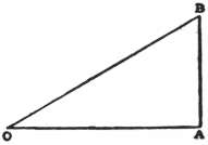
Fig. 1.

2. The guise in which variable quantities presented themselves to the mathematicians of the 17th century was that of the lengths of variable lines. This method of representing variable quantities dates from the 14th century, Geometrical representation of Variable Quantities. when it was employed by Nicole Oresme, who studied and afterwards taught at the Collège de Navarre in Paris from 1348 to 1361. He represented one of two variable quantities, e.g. the time that has elapsed since some epoch, by a length, called the “longitude,” measured along a particular line; and he represented the other of the two quantities, e.g. the temperature at the instant, by a length, called the “latitude,” measured at right angles to this line. He recognized that the variation of the temperature with the time was represented by the line, straight or curved, which joined the ends of all the lines of “latitude.” Oresme’s longitude and latitude were what we should now call the abscissa and ordinate. The same method was used later by many writers, among whom Johannes Kepler and Galileo Galilei may be mentioned. In Galileo’s investigation of the motion of falling bodies (1638) the abscissa OA represents the time during which a body has been falling, and the ordinate AB represents the velocity acquired during that time (see fig. 1). The velocity being proportional to the time, the “curve” obtained is a straight line OB, and Galileo showed that the distance through which the body has fallen is represented by the area of the triangle OAB.

The most prominent problems in regard to a curve were the problem of finding the points at which the ordinate is a maximum or a minimum, the problem of drawing a tangent to the curve at an assigned point, and the problem of The problems of Maxima and Minima, Tangents, and Quadratures. determining the area of the curve. The relation of the problem of maxima and minima to the problem of tangents was understood in the sense that maxima or minima arise when a certain equation has equal roots, and, when this is the case, the curves by which the problem is to be solved touch each other. The reduction of problems of maxima and minima to problems of contact was known to Pappus. The problem of finding the area of a curve was usually presented in a particular form in which it is called the “problem of quadratures.” It was sought to determine the area contained between the curve, the axis of abscissae and two ordinates, of which one was regarded as fixed and the other as variable. Galileo’s investigation may serve as an example. In that example the fixed ordinate vanishes. From this investigation it may be seen that before the invention of the infinitesimal calculus the introduction of a curve into discussions of the course of any phenomenon, and the problem of quadratures for that curve, were not exclusively of geometrical import; the purpose for which the area of a curve was sought was often to find something which is not an area—for instance, a length, or a volume or a centre of gravity.

3. The Greek geometers made little progress with the problem of tangents, but they devised methods for investigating the problem of quadratures. One of these methods was afterwards called the “method of exhaustions,” and Greek methods. the principle on which it is based was laid down in the lemma prefixed to the 12th book of Euclid’s Elements as follows: “If from the greater of two magnitudes there be taken more than its half, and from the remainder more than its half, and so on, there will at length remain a magnitude less than the smaller of the proposed magnitudes.” The method adopted by Archimedes was more general. It may be described as the enclosure of the magnitude to be evaluated between two others which can be brought by a definite process to differ from each other by less than any assigned magnitude. A simple example of its application is the 6th proposition of Archimedes’ treatise On the Sphere and Cylinder, in which it is proved that the area contained between a regular polygon inscribed in a circle and a similar polygon circumscribed to the same circle can be made less than any assigned area by increasing the number of sides of the polygon. The methods of Euclid and Archimedes were specimens of rigorous limiting processes (see Function). The new problems presented by the analytical geometry and natural philosophy of the 17th century led to new limiting processes.

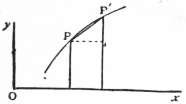
Fig. 2.

4. In the problem of tangents the new process may be described as follows. Let P, P′ be two points of a curve (see fig. 2). Let x, y be the coordinates of P, and x + Δx, y + Δy those of P′. The symbol Δx means “the difference of two Differentiation. x’s” and there is a like meaning for the symbol Δy. The fraction Δy/Δx is the trigonometrical tangent of the angle which the secant PP′ makes with the axis of x. Now let Δx be continually diminished towards zero, so that P′ continually approaches P. If the curve has a tangent at P the secant PP′ approaches a limiting position (see § 33 below). When this is the case the fraction Δy/Δx tends to a limit, and this limit is the trigonometrical tangent of the angle which the tangent at P to the curve makes with the axis of x. The limit is denoted by

dy .

dx

If the equation of the curve is of the form y = ƒ(x) where ƒ is a functional symbol (see Function), then

Δy = ƒ(x + Δx) − ƒ(x) ,

Δx Δx

and

dy = lim.Δx = 0 ƒ(x + Δx) − ƒ(x) .

dx Δx

The limit expressed by the right-hand member of this defining equation is often written

ƒ′(x),

and is called the “derived function” of ƒ(x), sometimes the “derivative” or “derivate” of ƒ(x). When the function ƒ(x) is a rational integral function, the division by Δx can be performed, and the limit is found by substituting zero for Δx in the quotient. For example, if ƒ(x) = x2, we have

ƒ(x + Δx) − ƒ(x) = (x + Δx)2 − x2 = 2xΔx + (Δx)2 ,

Δx Δx Δx

and

ƒ′(x) = 2x.

The process of forming the derived function of a given function is called differentiation. The fraction Δy/Δx is called the “quotient of differences,” and its limit dy/dx is called the “differential coefficient of y with respect to x.” The rules for forming differential coefficients constitute the differential calculus.

The problem of tangents is solved at one stroke by the formation of the differential coefficient; and the problem of maxima and minima is solved, apart from the discrimination of maxima from minima and some further refinements, by equating the differential coefficient to zero (see Maxima and Minima).

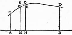
Fig. 3.

5. The problem of quadratures leads to a type of limiting process which may be described as follows: Let y = ƒ(x) be the equation of a curve, and let AC and BD be the ordinates of the points C and D (see fig. 3). Let a, b be the abscissae of these Integration. points. Let the segment AB be divided into a number of segments by means of intermediate points such as M, and let MN be one such segment. Let PM and QN be those ordinates of the curve which have M and N as their feet. On MN as base describe two rectangles, of which the heights are the greatest and least values of y which correspond to points on the arc PQ of the curve. In fig. 3 these are the rectangles RM, SN. Let the sum of the areas of such rectangles as RM be formed, and likewise the sum of the areas of such rectangles as SN. When the number of the points such as M is increased without limit, and the lengths of all the segments such as MN are diminished without limit, these two sums of areas tend to limits. When they tend to the same limit the curvilinear figure ACDB has an area, and the limit is the measure of this area (see § 33 below). The limit in question is the same whatever law may be adopted for inserting the points such as M between A and B, and for diminishing the lengths of the segments such as MN. Further, if P′ is any point on the arc PQ, and P′M′ is the ordinate of P′, we may construct a rectangle of which the height is P′M′ and the base is MN, and the limit of the sum of the areas of all such rectangles is the area of the figure as before. If x is the abscissa of P, x + Δx that of Q, x′ that of P′, the limit in question might be written

lim. Σba ƒ(x′) Δx,

where the letters a, b written below and above the sign of summation Σ indicate the extreme values of x. This limit is called “the definite integral of ƒ(x) between the limits a and b,” and the notation for it is

∫ba ƒ(x) dx.

The germs of this method of formulating the problem of quadratures are found in the writings of Archimedes. The method leads to a definition of a definite integral, but the direct application of it to the evaluation of integrals is in general difficult. Any process for evaluating a definite integral is a process of integration, and the rules for evaluating integrals constitute the integral calculus.

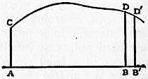
Fig. 4.

6. The chief of these rules is obtained by regarding the extreme ordinate BD as variable. Let ξ now denote the abscissa of B. The area A of the figure ACDB is represented by the Theorem of Inversion. integral ∫ξa ƒ(x)dx, and it is a function of ξ. Let BD be displaced to B′D′ so that ξ becomes ξ + δξ (see fig. 4). The area of the figure ACD′B′ is represented by the integral ∫ξ+Δξa ƒ(x)dx, and the increment ΔA of the area is given by the formula

ΔA = ∫ξ+Δξξ ƒ(x) dx,

which represents the area BDD′B′. This area is intermediate between those of two rectangles, having as a common base the segment BB′, and as heights the greatest and least ordinates of points on the arc DD′ of the curve. Let these heights be H and h. Then ΔA is intermediate between HΔξ and hΔξ, and the quotient of differences ΔA/Δξ is intermediate between H and h. If the function ƒ(x) is continuous at B (see Function), then, as Δξ is diminished without limit, H and h tend to BD, or ƒ(ξ), as a limit, and we have

dA = ƒ(ξ).

dξ

The introduction of the process of differentiation, together with the theorem here proved, placed the solution of the problem of quadratures on a new basis. It appears that we can always find the area A if we know a function F(x) which has ƒ(x) as its differential coefficient. If ƒ(x) is continuous between a and b, we can prove that

A = ∫ba ƒ(x) dx = F(b) − F(a).

When we recognize a function F(x) which has the property expressed by the equation

dF(x) = ƒ(x),

dx

we are said to integrate the function ƒ(x), and F(x) is called the indefinite integral of ƒ(x) with respect to x, and is written

∫ ƒ(x) dx.

7. In the process of § 4 the increment Δy is not in general equal to the product of the increment Δx and the derived Differentials. function ƒ′(x). In general we can write down an equation of the form

Δy = ƒ′(x) Δx + R,

in which R is different from zero when Δx is different from zero; and then we have not only

lim.Δx=0 R = 0,

but also

lim.Δx=0 R = 0.

Δx

We may separate Δy into two parts: the part ƒ′(x)Δx and the part R. The part ƒ′(x)Δx alone is useful for forming the differential coefficient, and it is convenient to give it a name. It is called the differential of ƒ(x), and is written dƒ(x), or dy when y is written for ƒ(x). When this notation is adopted dx is written instead of Δx, and is called the “differential of x,” so that we have

dƒ(x) = ƒ′(x) dx.

Thus the differential of an independent variable such as x is a finite difference; in other words it is any number we please. The differential of a dependent variable such as y, or of a function of the independent variable x, is the product of the differential of x and the differential coefficient or derived function. It is important to observe that the differential coefficient is not to be defined as the ratio of differentials, but the ratio of differentials is to be defined as the previously introduced differential coefficient. The differentials are either finite differences, or are so much of certain finite differences as are useful for forming differential coefficients.

Again let F(x) be the indefinite integral of a continuous function ƒ(x), so that we have

dF(x) = ƒ(x), ∫ba ƒ(x) dx = F(b) − F(a).

dx

When the points M of the process explained in § 5 are inserted between the points whose abscissae are a and b, we may take them to be n − 1 in number, so that the segment AB is divided into n segments. Let x1, x2, ... xn−1 be the abscissae of the points in order. The integral is the limit of the sum

ƒ(a) (x1 − a) + ƒ(x1) (x2 − x1) + ... + ƒ(xr) (xr+1 − xr) + ... + ƒ(xn−1) (b − xn−1),

every term of which is a differential of the form ƒ(x)dx. Further the integral is equal to the sum of differences

{F(x1) − F(a)} + {F(x2) − F(x1)} + ... + {F(xr+1) − F(xr)} + ... + {F(b) − F(xn−1)},

for this sum is F(b) − F(a). Now the difference F(xr+1) − F(xr) is not equal to the differential ƒ(xr) (xr+1 − xr), but the sum of the differences is equal to the limit of the sum of these differentials. The differential may be regarded as so much of the difference as is required to form the integral. From this point of view a differential is called a differential element of an integral, and the integral is the limit of the sum of differential elements. In like manner the differential element ydx of the area of a curve (§ 5) is not the area of the portion contained between two ordinates, however near together, but is so much of this area as need be retained for the purpose of finding the area of the curve by the limiting process described.

8. The notation of the infinitesimal calculus is intimately bound up with the notions of differentials and sums of elements. The letter Notation. Fundamental Artifice. “d” is the initial letter of the word differentia (difference) and the symbol ∫ is a conventionally written “S,” the initial letter of the word summa (sum or whole). The notation was introduced by Leibnitz (see §§ 25-27, below).

9. The fundamental artifice of the calculus is the artifice of forming differentials without first forming differential coefficients. From an equation containing x and y we can deduce a new equation, containing also Δx and Δy, by substituting x + Δx for x and y + Δy for y. If there is a differential coefficient of y with respect to x, then Δy can be expressed in the form φ.Δx + R, where lim.Δx=0 (R/Δx) = 0, as in § 7 above. The artifice consists in rejecting ab initio all terms of the equation which belong to R. We do not form R at all, but only φ·Δx, or φ.dx, which is the differential dy. In the same way, in all applications of the integral calculus to geometry or mechanics we form the element of an integral in the same way as the element of area y·dx is formed. In fig. 3 of § 5 the element of area y·dx is the area of the rectangle RM. The actual area of the curvilinear figure PQNM is greater than the area of this rectangle by the area of the curvilinear figure PQR; but the excess is less than the area of the rectangle PRQS, which is measured by the product of the numerical measures of MN and QR, and we have

lim.MN = 0 MN · QR = 0.

MN

Thus the artifice by which differential elements of integrals are formed is in principle the same as that by which differentials are formed without first forming differential coefficients.

10. This principle is usually expressed by introducing the notion of orders of small quantities. If x, y are two variable numbers which are Orders of small quantities. connected together by any relation, and if when x tends to zero y also tends to zero, the fraction y/x may tend to a finite limit. In this case x and y are said to be “of the same order.” When this is not the case we may have either

lim.x=0 x = 0,

y

or

lim.x=0 y = 0,

x

In the former case y is said to be “of a lower order” than x; in the latter case y is said to be “of a higher order” than x. In accordance with this notion we may say that the fundamental artifice of the infinitesimal calculus consists in the rejection of small quantities of an unnecessarily high order. This artifice is now merely an incident in the conduct of a limiting process, but in the 17th century, when limiting processes other than the Greek methods for quadratures were new, the introduction of the artifice was a great advance.

11. By the aid of this artifice, or directly by carrying out the appropriate limiting processes, we may obtain the Rules of Differentiation. rules by which differential coefficients are formed. These rules may be classified as “formal rules” and “particular results.” The formal rules may be stated as follows:—

(i.) The differential coefficient of a constant is zero.

(ii.) For a sum u + v + ... + z, where u, v, ... are functions of x,

d(u + v + ... + z) = du + dv + ... + dz .

dx dx dx dx

(iii.) For a product uv

d(uv) = u dv + v du .

dx dx dx

(iv.) For a quotient u/v

d(u/v) = ( v du − u dv ) / v2.

dx dx dx

(v.) For a function of a function, that is to say, for a function y expressed in terms of a variable z, which is itself expressed as a function of x,

dy = dy · dz .

dx dz dx

In addition to these formal rules we have particular results as to the differentiation of simple functions. The most important results are written down in the following table:—

y dy/dx

xn nxn−1 for all values of n

logax x-1 logae

ax ax logea

sin x cos x

cos x −sin x

sin−1x (1 − x2)−1/2

tan−1x (1 + x2)−1

Each of the formal rules, and each of the particular results in the table, is a theorem of the differential calculus. All functions (or rather expressions) which can be made up from those in the table by a finite number of operations of addition, subtraction, multiplication or division can be differentiated by the formal rules. All such functions are called explicit functions. In addition to these we have implicit functions, or such as are determined by an equation containing two variables when the equation cannot be solved so as to exhibit the one variable expressed in terms of the other. We have also functions of several variables. Further, since the derived function of a given function is itself a function, we may seek to differentiate it, and thus there arise the second and higher differential coefficients. We postpone for the present the problems of differential calculus which arise from these considerations. Again, we may have explicit functions which are expressed as the results of limiting operations, or by the limits of the results obtained by performing an infinite number of algebraic operations upon the simple functions. For the problem of differentiating such functions reference may be made to Function.

12. The processes of the integral calculus consist largely in transformations Indefinite Integrals. of the functions to be integrated into such forms that they can be recognized as differential coefficients of functions which have previously been differentiated. Corresponding to the results in the table of § 11 we have those in the following table:—

ƒ(x) ∫ƒ(x)dx

xn xn+1 / (n + 1) for all values of n except −1

1/x loge x

eax a−1eax

cos x sin x

sin x −cos x

(a2 − x2)−1/2 sin−1 (x/a)

1 / (a2 + x2) (1/a) tan−1 (x/a)

The formal rules of § 11 give us means for the transformation of integrals into recognizable forms. For example, the rule (ii.) for a sum leads to the result that the integral of a sum of a finite number of terms is the sum of the integrals of the several terms. The rule (iii.) for a product leads to the method of integration by parts. The rule (v.) for a function of a function leads to the method of substitution (see § 48 below.)

II. History.

13. The new limiting processes which were introduced in the development of the higher analysis were in the first instance related to problems of the integral calculus. Johannes Kepler in his Astronomia nova ... de motibus stellae Martis Kepler’s methods of Integration. (1609) stated his laws of planetary motion, to the effect that the orbits of the planets are ellipses with the sun at a focus, and that the radii vectores drawn from the sun to the planets describe equal areas in equal times. From these statements it is to be concluded that Kepler could measure the areas of focal sectors of an ellipse. When he made out these laws there was no method of evaluating areas except the Greek methods. These methods would have sufficed for the purpose, but Kepler invented his own method. He regarded the area as measured by the “sum of the radii” drawn from the focus, and he verified his laws of planetary motion by actually measuring a large number of radii of the orbit, spaced according to a rule, and adding their lengths.

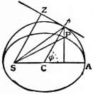
Fig. 5.

He had observed that the focal radius vector SP (fig. 5) is equal to the perpendicular SZ drawn from S to the tangent at p to the auxiliary circle, and he had further established the theorem which we should now express in the form—the differential element of the area ASp as Sp turns about S, is equal to the product of SZ and the differential adφ, where a is the radius of the auxiliary circle, and φ is the angle ACp, that is the eccentric angle of P on the ellipse. The area ASP bears to the area ASp the ratio of the minor to the major axis, a result known to Archimedes. Thus Kepler’s radii are spaced according to the rule that the eccentric angles of their ends are equidifferent, and his “sum of radii” is proportional to the expression which we should now write

∫φ0 (a + ae cos φ) dφ,

where e is the eccentricity. Kepler evaluated the sum as proportional to φ + e sin φ.

Kepler soon afterwards occupied himself with the volumes of solids. The vintage of the year 1612 was extraordinarily abundant, and the question of the cubic content of wine casks was brought under his notice. This fact accounts for the title of his work, Nova stereometria doliorum; accessit stereometriae Archimedeae supplementum (1615). In this treatise he regarded solid bodies as being made up, as it were (veluti), of “infinitely” many “infinitely” small cones or “infinitely” thin disks, and he used the notion of summing the areas of the disks in the way he had previously used the notion of summing the focal radii of an ellipse.

14. In connexion with the early history of the calculus it must not be forgotten that the method by which logarithms were invented (1614) was effectively a method of infinitesimals. Natural logarithms were not invented Logarithms. as the indices of a certain base, and the notation e for the base was first introduced by Euler more than a century after the invention. Logarithms were introduced as numbers which increase in arithmetic progression when other related numbers increase in geometric progression. The two sets of numbers were supposed to increase together, one at a uniform rate, the other at a variable rate, and the increments were regarded for purposes of calculation as very small and as accruing discontinuously.

15. Kepler’s methods of integration, for such they must be called, were the origin of Bonaventura Cavalieri’s theory of the summation of indivisibles. The notion of a continuum, such as the area within a closed curve, Cavalieri’s Indivisibles. as being made up of indivisible parts, “atoms” of area, if the expression may be allowed, is traceable to the speculations of early Greek philosophers; and although the nature of continuity was better understood by Aristotle and many other ancient writers yet the unsound atomic conception was revived in the 13th century and has not yet been finally uprooted. It is possible to contend that Cavalieri did not himself hold the unsound doctrine, but his writing on this point is rather obscure. In his treatise Geometria indivisibilibus continuorum nova quadam ratione promota (1635) he regarded a plane figure as generated by a line moving so as to be always parallel to a fixed line, and a solid figure as generated by a plane moving so as to be always parallel to a fixed plane; and he compared the areas of two plane figures, or the volumes of two solids, by determining the ratios of the sums of all the indivisibles of which they are supposed to be made up, these indivisibles being segments of parallel lines equally spaced in the case of plane figures, and areas marked out upon parallel planes equally spaced in the case of solids. By this method Cavalieri was able to effect numerous integrations relating to the areas of portions of conic sections and the volumes generated by the revolution of these portions about various axes. At a later date, and partly in answer to an attack made upon him by Paul Guldin, Cavalieri published a treatise entitled Exercitationes geometricae sex (1647), in which he adapted his method to the determination of centres of gravity, in particular for solids of variable density.

Among the results which he obtained is that which we should now write

∫x0 xm dx = xm+1 , (m integral).

m + 1

He regarded the problem thus solved as that of determining the sum of the mth powers of all the lines drawn across a parallelogram parallel to one of its sides.

At this period scientific investigators communicated their results to one another through one or more intermediate persons. Such intermediaries were Pierre de Carcavy and Pater Marin Mersenne; and among the writers thus Successors of Cavalieri. in communication were Bonaventura Cavalieri, Christiaan Huygens, Galileo Galilei, Giles Personnier de Roberval, Pierre de Fermat, Evangelista Torricelli, and a little later Blaise Pascal; but the letters of Carcavy or Mersenne would probably come into the hands of any man who was likely to be interested in the matters discussed. It often happened that, when some new method was invented, or some new result obtained, the method or result was quickly known to a wide circle, although it might not be printed until after the lapse of a long time. When Cavalieri was printing his two treatises there was much discussion of the problem of quadratures. Roberval (1634) regarded an area as made up of “infinitely” many “infinitely” narrow strips, each of which may be considered to be a rectangle, and he had similar ideas in regard to lengths and volumes. He knew how to approximate to the quantity which we express by ∫10 xmdx by the process of forming the sum

0m + 1m + 2m + ... (n − 1)m ,

nm+1

and he claimed to be able to prove that this sum tends to 1/(m + 1), as n increases for all positive integral values of m. The method of integrating xm by forming this sum was found also by Fermat (1636), who stated expressly that he Fermat’s method of Integration. arrived at it by generalizing a method employed by Archimedes (for the cases m = 1 and m = 2) in his books on Conoids and Spheroids and on Spirals (see T. L. Heath, The Works of Archimedes, Cambridge, 1897). Fermat extended the result to the case where m is fractional (1644), and to the case where m is negative. This latter extension and the proofs were given in his memoir, Proportionis geometricae in quadrandis parabolis et hyperbolis usus, which appears to have received a final form before 1659, although not published until 1679. Fermat did not use fractional or negative indices, but he regarded his problems as the quadratures of parabolas and hyperbolas of various orders. His method was to divide the interval of integration into parts by means of intermediate points the abscissae of which are in geometric progression. In the process of § 5 above, the points M must be chosen according to this rule. This restrictive condition being understood, we may say that Fermat’s formulation of the problem of quadratures is the same as our definition of a definite integral.

The result that the problem of quadratures could be solved for any curve whose equation could be expressed in the form

y = xm (m ≠ −1),

or in the form

y = a1 xm1 + a2 xm2 + ... + an xmn,

where none of the indices is equal to −1, was used by John Various Integrations. Wallis in his Arithmetica infinitorum (1655) as well as by Fermat (1659). The case in which m = −1 was that of the ordinary rectangular hyperbola; and Gregory of St Vincent in his Opus geometricum quadraturae circuli et sectionum coni (1647) had proved by the method of exhaustions that the area contained between the curve, one asymptote, and two ordinates parallel to the other asymptote, increases in arithmetic progression as the distance between the ordinates (the one nearer to the centre being kept fixed) increases in geometric progression. Fermat described his method of integration as a logarithmic method, and thus it is clear that the relation between the quadrature of the hyperbola and logarithms was understood although it was not expressed analytically. It was not very long before the relation was used for the calculation of logarithms by Nicolaus Mercator in his Logarithmotechnia (1668). He began by writing the equation of the curve in the form y = 1/(1 + x), expanded this expression in powers of x by the method of division, and integrated it term by term in accordance with the well-understood rule for finding the quadrature of a curve given by such an equation as that written at the foot of p. 325.

By the middle of the 17th century many mathematicians could perform integrations. Very many particular results had been obtained, and applications of them had been Integration before the Integral Calculus. made to the quadrature of the circle and other conic sections, and to various problems concerning the lengths of curves, the areas they enclose, the volumes and superficial areas of solids, and centres of gravity. A systematic account of the methods then in use was given, along with much that was original on his part, by Blaise Pascal in his Lettres de Amos Dettonville sur quelques-unes de ses inventions en géométrie (1659).

16. The problem of maxima and minima and the problem of tangents had also by the same time been effectively solved. Oresme in the 14th century knew that at a point where the ordinate of a curve is a maximum or a minimum Fermat’s methods of Differentiation. its variation from point to point of the curve is slowest; and Kepler in the Stereometria doliorum remarked that at the places where the ordinate passes from a smaller value to the greatest value and then again to a smaller value, its variation becomes insensible. Fermat in 1629 was in possession of a method which he then communicated to one Despagnet of Bordeaux, and which he referred to in a letter to Roberval of 1636. He communicated it to René Descartes early in 1638 on receiving a copy of Descartes’s Géométrie (1637), and with it he sent to Descartes an account of his methods for solving the problem of tangents and for determining centres of gravity.

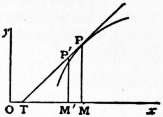
Fig. 6.

Fermat’s method for maxima and minima is essentially our method. Expressed in a more modern notation, what he did was to begin by connecting the ordinate y and the abscissa x of a point of a curve by an equation which holds at all points of the curve, then to subtract the value of y in terms of x from the value obtained by substituting x + E for x, then to divide the difference by E, to put E = 0 in the quotient, and to equate the quotient to zero. Thus he differentiated with respect to x and equated the differential coefficient to zero.

Fermat’s method for solving the problem of tangents may be explained as follows:—Let (x, y) be the coordinates of a point P of a curve, (x′, y′), those of a neighbouring point P′ on the tangent at P, and let MM′ = E (fig. 6).

From the similarity of the triangles P′TM′, PTM we have

y′ : A − E = y : A,

where A denotes the subtangent TM. The point P′ being near the curve, we may substitute in the equation of the curve x − E for x and (yA − yE)/A for y. The equation of the curve is approximately satisfied. If it is taken to be satisfied exactly, the result is an equation of the form φ(x, y, A, E) = 0, the left-hand member of which is divisible by E. Omitting the factor E, and putting E = 0 in the remaining factor, we have an equation which gives A. In this problem of tangents also Fermat found the required result by a process equivalent to differentiation.

Fermat gave several examples of the application of his method; among them was one in which he showed that he could differentiate very complicated irrational functions. For such functions his method was to begin by obtaining a rational equation. In rationalizing equations Fermat, in other writings, used the device of introducing new variables, but he did not use this device to simplify the process of differentiation. Some of his results were published by Pierre Hérigone in his Supplementum cursus mathematici (1642). His communication to Descartes was not published in full until after his death (Fermat, Opera varia, 1679). Methods similar to Fermat’s were devised by René de Sluse (1652) for tangents, and by Johannes Hudde (1658) for maxima and minima. Other methods for the solution of the problem of tangents were devised by Roberval and Torricelli, and published almost simultaneously in 1644. These methods were founded upon the composition of motions, the theory of which had been taught by Galileo (1638), and, less completely, by Roberval (1636). Roberval and Torricelli could construct the tangents of many curves, but they did not arrive at Fermat’s artifice. This artifice is that which we have noted in § 10 as the fundamental artifice of the infinitesimal calculus.

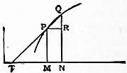
Fig. 7.

17. Among the comparatively few mathematicians who before 1665 could perform differentiations was Isaac Barrow. In his book entitled Lectiones opticae et geometricae, written apparently in 1663, 1664, and published in Barrow’s Differential Triangle. 1669, 1670, he gave a method of tangents like that of Roberval and Torricelli, compounding two velocities in the directions of the axes of x and y to obtain a resultant along the tangent to a curve. In an appendix to this book he gave another method which differs from Fermat’s in the introduction of a differential equivalent to our dy as well as dx. Two neighbouring ordinates PM and QN of a curve (fig. 7) are regarded as containing an indefinitely small (indefinite parvum) arc, and PR is drawn parallel to the axis of x. The tangent PT at P is regarded as identical with the secant PQ, and the position of the tangent is determined by the similarity of the triangles PTM, PQR. The increments QR, PR of the ordinate and abscissa are denoted by a and e; and the ratio of a to e is determined by substituting x + e for x and y + a for y in the equation of the curve, rejecting all terms which are of order higher than the first in a and e, and omitting the terms which do not contain a or e. This process is equivalent to differentiation. Barrow appears to have invented it himself, but to have put it into his book at Newton’s request. The triangle PQR is sometimes called “Barrow’s differential triangle.”

The reciprocal relation between differentiation and integration (§ 6) was first observed explicitly by Barrow in the book cited above. If the quadrature of a curve y = ƒ(x) is known, so that the area up to the ordinate x is given by F(x), the curve Barrow’s Inversion-theorem. y = F(x) can be drawn, and Barrow showed that the subtangent of this curve is measured by the ratio of its ordinate to the ordinate of the original curve. The curve y = F(x) is often called the “quadratrix” of the original curve; and the result has been called “Barrow’s inversion-theorem.” He did not use it as we do for the determination of quadratures, or indefinite integrals, but for the solution of problems of the kind which were then called “inverse problems of tangents.” In these problems it was sought to determine a curve from some property of its tangent, e.g. the property that the subtangent is proportional to the square of the abscissa. Such problems are now classed under “differential equations.” When Barrow wrote, quadratures were familiar and differentiation unfamiliar, just as hyperbolas were trusted while logarithms were strange. The functional notation was not invented till long afterwards (see Function), and the want of it is felt in reading all the mathematics of the 17th century.

18. The great secret which afterwards came to be called the “infinitesimal calculus” was almost discovered by Fermat, and still more nearly by Barrow. Barrow went farther than Fermat in the theory of differentiation, though not in the Nature of the discovery called the Infinitesimal Calculus. practice, for he compared two increments; he went farther in the theory of integration, for he obtained the inversion-theorem. The great discovery seems to consist partly in the recognition of the fact that differentiation, known to be a useful process, could always be performed, at least for the functions then known, and partly in the recognition of the fact that the inversion-theorem could be applied to problems of quadrature. By these steps the problem of tangents could be solved once for all, and the operation of integration, as we call it, could be rendered systematic. A further step was necessary in order that the discovery, once made, should become accessible to mathematicians in general; and this step was the introduction of a suitable notation. The definite abandonment of the old tentative methods of integration in favour of the method in which this operation is regarded as the inverse of differentiation was especially the work of Isaac Newton; the precise formulation of simple rules for the process of differentiation in each special case, and the introduction of the notation which has proved to be the best, were especially the work of Gottfried Wilhelm Leibnitz. This statement remains true although Newton invented a systematic notation, and practised differentiation by rules equivalent to those of Leibnitz, before Leibnitz had begun to work upon the subject, and Leibnitz effected integrations by the method of recognizing differential coefficients before he had had any opportunity of becoming acquainted with Newton’s methods.

19. Newton was Barrow’s pupil, and he knew to start with in 1664 all that Barrow knew, and that was practically all that was known about the subject at that time. His original thinking on the subject dates from the year Newton’s investigations. of the great plague (1665-1666), and it issued in the invention of the “Calculus of Fluxions,” the principles and methods of which were developed by him in three tracts entitled De analysi per aequationes numero terminorum infinitas, Methodus fluxionum et serierum infinitarum, and De quadratura curvarum. None of these was published until long after they were written. The Analysis per aequationes was composed in 1666, but not printed until 1711, when it was published by William Jones. The Methodus fluxionum was composed in 1671 but not printed till 1736, nine years after Newton’s death, when an English translation was published by John Colson. In Horsley’s edition of Newton’s works it bears the title Geometria analytica. The Quadratura appears to have been composed in 1676, but was first printed in 1704 as an appendix to Newton’s Opticks.

20. The tract De Analysi per aequationes ... was sent by Newton to Barrow, who sent it to John Collins with a request that it might be made known. One way of making it known would have been to print it in the Philosophical Transactions Newton’s method of Series. of the Royal Society, but this course was not adopted. Collins made a copy of the tract and sent it to Lord Brouncker, but neither of them brought it before the Royal Society. The tract contains a general proof of Barrow’s inversion-theorem which is the same in principle as that in § 6 above. In this proof and elsewhere in the tract a notation is introduced for the momentary increment (momentum) of the abscissa or area of a curve; this “moment” is evidently meant to represent a moment of time, the abscissa representing time, and it is effectively the same as our differential element—the thing that Fermat had denoted by E, and Barrow by e, in the case of the abscissa. Newton denoted the moment of the abscissa by o, that of the area z by ov. He used the letter v for the ordinate y, thus suggesting that his curve is a velocity-time graph such as Galileo had used. Newton gave the formula for the area of a curve v = xm(m ± −1) in the form z = xm+1/(m + 1). In the proof he transformed this formula to the form zn = cn xp, where n and p are positive integers, substituted x + o for x and z + ov for z, and expanded by the binomial theorem for a positive integral exponent, thus obtaining the relation

zn + nzn−1 ov + ... = cn (xp + pxp−1 o + ...),

from which he deduced the relation

nzn−1 v = cn pxp−1

by omitting the equal terms zn and cnxp and dividing the remaining terms by o, tacitly putting o = 0 after division. This relation is the same as v = xm. Newton pointed out that, conversely, from the relation v = xm the relation z = xm+1 / (m + 1) follows. He applied his formula to the quadrature of curves whose ordinates can be expressed as the sum of a finite number of terms of the form axm; and gave examples of its application to curves in which the ordinate is expressed by an infinite series, using for this purpose the binomial theorem for negative and fractional exponents, that is to say, the expansion of (1 + x)n in an infinite series of powers of x. This theorem he had discovered; but he did not in this tract state it in a general form or give any proof of it. He pointed out, however, how it may be used for the solution of equations by means of infinite series. He observed also that all questions concerning lengths of curves, volumes enclosed by surfaces, and centres of gravity, can be formulated as problems of quadratures, and can thus be solved either in finite terms or by means of infinite series. In the Quadratura (1676) the method of integration which is founded upon the inversion-theorem was carried out systematically. Among other results there given is the quadrature of curves expressed by equations of the form y = xn (a + bxm)p; this has passed into text-books under the title “integration of binomial differentials” (see § 49). Newton announced the result in letters to Collins and Oldenburg of 1676.

21. In the Methodus fluxionum (1671) Newton introduced his characteristic notation. He regarded variable quantities as generated by the motion of a point, or line, or plane, and called the generated quantity a “fluent” and its rate of generation Newton’s method of Fluxions. a “fluxion.” The fluxion of a fluent x is represented by x, and its moment, or “infinitely” small increment accruing in an “infinitely” short time, is represented by ẋo. The problems of the calculus are stated to be (i.) to find the velocity at any time when the distance traversed is given; (ii.) to find the distance traversed when the velocity is given. The first of these leads to differentiation. In any rational equation containing x and y the expressions x + ẋo and y +ẏo are to be substituted for x and y, the resulting equation is to be divided by o, and afterwards o is to be omitted. In the case of irrational functions, or rational functions which are not integral, new variables are introduced in such a way as to make the equations contain rational integral terms only. Thus Newton’s rules of differentiation would be in our notation the rules (i.), (ii.), (v.) of § 11, together with the particular result which we write

dxm = mxm−1, (m integral).

dx

a result which Newton obtained by expanding (x = ẋo)m by the binomial theorem. The second problem is the problem of integration, and Newton’s method for solving it was the method of series founded upon the particular result which we write

∫ xm dx = xm+1 .

m + 1

Newton added applications of his methods to maxima and minima, tangents and curvature. In a letter to Collins of date 1672 Newton stated that he had certain methods, and he described certain results which he had found by using them. These methods and results are those which are to be found in the Methodus fluxionum; but the letter makes no mention of fluxions and fluents or of the characteristic notation. The rule for tangents is said in the letter to be analogous to de Sluse’s, but to be applicable to equations that contain irrational terms.

22. Newton gave the fluxional notation also in the tract De Quadratura curvarum (1676), and he there added to it notation for the higher differential coefficients and for indefinite integrals, as we call them. Just as x, y, z, ... are fluents Publication of the Fluxional Notation. of which ẋ, ẏ, ̇z, ... are the fluxions, so ẋ, ẏ, ̇z, ... can be treated as fluents of which the fluxions may be denoted by ẍ, ̈y, ̈z,... In like manner the fluxions of these may be denoted by ẍ, ̈y, ̈z, ... and so on. Again x, y, z, ... may be regarded as fluxions of which the fluents may be denoted by ́x, ́y, ́z, ... and these again as fluxions of other quantities denoted by ̋x, ̋y, ̋z, ... and so on. No use was made of the notation ́x, ̋x, ... in the course of the tract. The first publication of the fluxional notation was made by Wallis in the second edition of his Algebra (1693) in the form of extracts from communications made to him by Newton in 1692. In this account of the method the symbols 0, ẋ, ẍ, ... occur, but not the symbols ́x, ̋x, .... Wallis’s treatise also contains Newton’s formulation of the problems of the calculus in the words Data aequatione fluentes quotcumque quantitates involvente fluxiones invenire et vice versa (“an equation containing any number of fluent quantities being given, to find their fluxions and vice versa”). In the Philosophiae naturalis principia mathematica (1687), commonly called the “Principia,” the words “fluxion” and “moment” occur in a lemma in the second book; but the notation which is characteristic of the calculus of fluxions is nowhere used.

23. It is difficult to account for the fragmentary manner of publication of the Fluxional Calculus and for the long delays which took place. At the time (1671) when Newton composed the Methodus fluxionum he contemplated Retarded Publication of the method of Fluxions. bringing out an edition of Gerhard Kinckhuysen’s treatise on algebra and prefixing his tract to this treatise. In the same year his “Theory of Light and Colours” was published in the Philosophical Transactions, and the opposition which it excited led to the abandonment of the project with regard to fluxions. In 1680 Collins sought the assistance of the Royal Society for the publication of the tract, and this was granted in 1682. Yet it remained unpublished. The reason is unknown; but it is known that about 1679, 1680, Newton took up again the studies in natural philosophy which he had intermitted for several years, and that in 1684 he wrote the tract De motu which was in some sense a first draft of the Principia, and it may be conjectured that the fluxions were held over until the Principia should be finished. There is also reason to think that Newton had become dissatisfied with the arguments about infinitesimals on which his calculus was based. In the preface to the De quadratura curvarum (1704), in which he describes this tract as something which he once wrote (“olim scripsi”) he says that there is no necessity to introduce into the method of fluxions any argument about infinitely small quantities; and in the Principia (1687) he adopted instead of the method of fluxions a new method, that of “Prime and Ultimate Ratios.” By the aid of this method it is possible, as Newton knew, and as was afterwards seen by others, to found the calculus of fluxions on an irreproachable method of limits. For the purpose of explaining his discoveries in dynamics and astronomy Newton used the method of limits only, without the notation of fluxions, and he presented all his results and demonstrations in a geometrical form. There is no doubt that he arrived at most of his theorems in the first instance by using the method of fluxions. Further evidence of Newton’s dissatisfaction with arguments about infinitely small quantities is furnished by his tract Methodus diferentialis, published in 1711 by William Jones, in which he laid the foundations of the “Calculus of Finite Differences.”

24. Leibnitz, unlike Newton, was practically a self-taught mathematician. He seems to have been first attracted to mathematics as a means of symbolical expression, and on the occasion of his first visit to London, early in Leibnitz’s course of discovery. 1673, he learnt about the doctrine of infinite series which James Gregory, Nicolaus Mercator, Lord Brouncker and others, besides Newton, had used in their investigations. It appears that he did not on this occasion become acquainted with Collins, or see Newton’s Analysis per aequationes, but he purchased Barrow’s Lectiones. On returning to Paris he made the acquaintance of Huygens, who recommended him to read Descartes’ Géométrie. He also read Pascal’s Lettres de Dettonville, Gregory of St Vincent’s Opus geometricum, Cavalieri’s Indivisibles and the Synopsis geometrica of Honoré Fabri, a book which is practically a commentary on Cavalieri; it would never have had any importance but for the influence which it had on Leibnitz’s thinking at this critical period. In August of this year (1673) he was at work upon the problem of tangents, and he appears to have made out the nature of the solution—the method involved in Barrow’s differential triangle—for himself by the aid of a diagram drawn by Pascal in a demonstration of the formula for the area of a spherical surface. He saw that the problem of the relation between the differences of neighbouring ordinates and the ordinates themselves was the important problem, and then that the solution of this problem was to be effected by quadratures. Unlike Newton, who arrived at differentiation and tangents through integration and areas, Leibnitz proceeded from tangents to quadratures. When he turned his attention to quadratures and indivisibles, and realized the nature of the process of finding areas by summing “infinitesimal” rectangles, he proposed to replace the rectangles by triangles having a common vertex, and obtained by this method the result which we write

1⁄4π = 1 − 1⁄3 + 1⁄5 − 1⁄7 + ...

In 1674 he sent an account of his method, called “transmutation,” along with this result to Huygens, and early in 1675 he sent it to Henry Oldenburg, secretary of the Royal Society, with inquiries as to Newton’s discoveries in regard to quadratures. In October of 1675 he had begun to devise a symbolical notation for quadratures, starting from Cavalieri’s indivisibles. At first he proposed to use the word omnia as an abbreviation for Cavalieri’s “sum of all the lines,” thus writing omnia y for that which we write “∫ ydx,” but within a day or two he wrote “∫ y”. He regarded the symbol “∫” as representing an operation which raises the dimensions of the subject of operation—a line becoming an area by the operation—and he devised his symbol “d” to represent the inverse operation, by which the dimensions are diminished. He observed that, whereas “∫” represents “sum,” “d” represents “difference.” His notation appears to have been practically settled before the end of 1675, for in November he wrote ∫ ydy = ½ y2, just as we do now.

25. In July of 1676 Leibnitz received an answer to his inquiry in regard to Newton’s methods in a letter written by Newton to Oldenburg. In this letter Newton gave a general statement of the binomial theorem and many results Correspondence of Newton and Leibnitz. relating to series. He stated that by means of such series he could find areas and lengths of curves, centres of gravity and volumes and surfaces of solids, but, as this would take too long to describe, he would illustrate it by examples. He gave no proofs. Leibnitz replied in August, stating some results which he had obtained, and which, as it seemed, could not be obtained easily by the method of series, and he asked for further information. Newton replied in a long letter to Oldenburg of the 24th of October 1676. In this letter he gave a much fuller account of his binomial theorem and indicated a method of proof. Further he gave a number of results relating to quadratures; they were afterwards printed in the tract De quadratura curvarum. He gave many other results relating to the computation of natural logarithms and other calculations in which series could be used. He gave a general statement, similar to that in the letter to Collins, as to the kind of problems relating to tangents, maxima and minima, &c., which he could solve by his method, but he concealed his formulation of the calculus in an anagram of transposed letters. The solution of the anagram was given eleven years later in the Principia in the words we have quoted from Wallis’s Algebra. In neither of the letters to Oldenburg does the characteristic notation of the fluxional calculus occur, and the words “fluxion” and “fluent” occur only in anagrams of transposed letters. The letter of October 1676 was not despatched until May 1677, and Leibnitz answered it in June of that year. In October 1676 Leibnitz was in London, where he made the acquaintance of Collins and read the Analysis per aequationes, and it seems to have been supposed afterwards that he then read Newton’s letter of October 1676, but he left London before Oldenburg received this letter. In his answer of June 1677 Leibnitz gave Newton a candid account of his differential calculus, nearly in the form in which he afterwards published it, and explained how he used it for quadratures and inverse problems of tangents. Newton never replied.

26. In the Acta eruditorum of 1684 Leibnitz published a short memoir entitled Nova methodus pro maximis et minimis, itemque tangentibus, quae nec fractas nec irrationales quantitates moratur, et singulare pro illis calculi genus. Leibnitz’s Differential Calculus. In this memoir the differential dx of a variable x, considered as the abscissa of a point of a curve, is said to be an arbitrary quantity, and the differential dy of a related variable y, considered as the ordinate of the point, is defined as a quantity which has to dx the ratio of the ordinate to the subtangent, and rules are given for operating with differentials. These are the rules for forming the differential of a constant, a sum (or difference), a product, a quotient, a power (or root). They are equivalent to our rules (i.)-(iv.) of § 11 and the particular result

d(xm) = mxm−1 dx.

The rule for a function of a function is not stated explicitly but is illustrated by examples in which new variables are introduced, in much the same way as in Newton’s Methodus fluxionum. In connexion with the problem of maxima and minima, it is noted that the differential of y is positive or negative according as y increases or decreases when x increases, and the discrimination of maxima from minima depends upon the sign of ddy, the differential of dy. In connexion with the problem of tangents the differentials are said to be proportional to the momentary increments of the abscissa and ordinate. A tangent is defined as a line joining two “infinitely” near points of a curve, and the “infinitely” small distances (e.g., the distance between the feet of the ordinates of such points) are said to be expressible by means of the differentials (e.g., dx). The method is illustrated by a few examples, and one example is given of its application to “inverse problems of tangents.” Barrow’s inversion-theorem and its application to quadratures are not mentioned. No proofs are given, but it is stated that they can be obtained easily by any one versed in such matters. The new methods in regard to differentiation which were contained in this memoir were the use of the second differential for the discrimination of maxima and minima, and the introduction of new variables for the purpose of differentiating complicated expressions. A greater novelty was the use of a letter (d), not as a symbol for a number or magnitude, but as a symbol of operation. None of these novelties account for the far-reaching effect which this memoir has had upon the development of mathematical analysis. This effect was a consequence of the simplicity and directness with which the rules of differentiation were stated. Whatever indistinctness might be felt to attach to the symbols, the processes for solving problems of tangents and of maxima and minima were reduced once for all to a definite routine.

27. This memoir was followed in 1686 by a second, entitled De Geometria recondita et analysi indivisibilium atque infinitorum, in which Leibnitz described the method of using his new differential calculus for the problem of quadratures. Development of the Calculus. This was the first publication of the notation ∫ ydx. The new method was called calculus summatorius. The brothers Jacob (James) and Johann (John) Bernoulli were able by 1690 to begin to make substantial contributions to the development of the new calculus, and Leibnitz adopted their word “integral” in 1695, they at the same time adopting his symbol “∫.” In 1696 the marquis de l’Hospital published the first treatise on the differential calculus with the title Analyse des infiniment petits pour l’intelligence des lignes courbes. The few references to fluxions in Newton’s Principia (1687) must have been quite unintelligible to the mathematicians of the time, and the publication of the fluxional notation and calculus by Wallis in 1693 was too late to be effective. Fluxions had been supplanted before they were introduced.

The differential calculus and the integral calculus were rapidly developed in the writings of Leibnitz and the Bernoullis. Leibnitz (1695) was the first to differentiate a logarithm and an exponential, and John Bernoulli was the first to recognize the property possessed by an exponential (ax) of becoming infinitely great in comparison with any power (xn) when x is increased indefinitely. Roger Cotes (1722) was the first to differentiate a trigonometrical function. A great development of infinitesimal methods took place through the founding in 1696-1697 of the “Calculus of Variations” by the brothers Bernoulli.

28. The famous dispute as to the priority of Newton and Leibnitz in the invention of the calculus began in 1699 through the publication by Nicolas Fatio de Duillier of a tract in which he stated that Newton was not only the Dispute concerning Priority. first, but by many years the first inventor, and insinuated that Leibnitz had stolen it. Leibnitz in his reply (Acta Eruditorum, 1700) cited Newton’s letters and the testimony which Newton had rendered to him in the Principia as proofs of his independent authorship of the method. Leibnitz was especially hurt at what he understood to be an endorsement of Duillier’s attack by the Royal Society, but it was explained to him that the apparent approval was an accident. The dispute was ended for a time. On the publication of Newton’s tract De quadratura curvarum, an anonymous review of it, written, as has since been proved, by Leibnitz, appeared in the Acta Eruditorum, 1705. The anonymous reviewer said: “Instead of the Leibnitzian differences Newton uses and always has used fluxions ... just as Honoré Fabri in his Synopsis Geometrica substituted steps of movements for the method of Cavalieri.” This passage, when it became known in England, was understood not merely as belittling Newton by comparing him with the obscure Fabri, but also as implying that he had stolen his calculus of fluxions from Leibnitz. Great indignation was aroused; and John Keill took occasion, in a memoir on central forces which was printed in the Philosophical Transactions for 1708, to affirm that Newton was without doubt the first inventor of the calculus, and that Leibnitz had merely changed the name and mode of notation. The memoir was published in 1710. Leibnitz wrote in 1711 to the secretary of the Royal Society (Hans Sloane) requiring Keill to retract his accusation. Leibnitz’s letter was read at a meeting of the Royal Society, of which Newton was then president, and Newton made to the society a statement of the course of his invention of the fluxional calculus with the dates of particular discoveries. Keill was requested by the society “to draw up an account of the matter under dispute and set it in a just light.” In his report Keill referred to Newton’s letters of 1676, and said that Newton had there given so many indications of his method that it could have been understood by a person of ordinary intelligence. Leibnitz wrote to Sloane asking the society to stop these unjust attacks of Keill, asserting that in the review in the Acta Eruditorum no one had been injured but each had received his due, submitting the matter to the equity of the Royal Society, and stating that he was persuaded that Newton himself would do him justice. A committee was appointed by the society to examine the documents and furnish a report. Their report, presented in April 1712, concluded as follows:

“The differential method is one and the same with the method of fluxions, excepting the name and mode of notation; Mr Leibnitz calling those quantities differences which Mr Newton calls moments or fluxions, and marking them with the letter d, a mark not used by Mr Newton. And therefore we take the proper question to be, not who invented this or that method, but who was the first inventor of the method; and we believe that those who have reputed Mr Leibnitz the first inventor, knew little or nothing of his correspondence with Mr Collins and Mr Oldenburg long before; nor of Mr Newton’s having that method above fifteen years before Mr. Leibnitz began to publish it in the Acta Eruditorum of Leipzig. For which reasons we reckon Mr Newton the first inventor, and are of opinion that Mr Keill, in asserting the same, has been no ways injurious to Mr Leibnitz.”

The report with the letters and other documents was printed (1712) under the title Commercium Epistolicum D. Johannis Collins et aliorum de analysi promota, jussu Societatis Regiae in lucem editum, not at first for publication. An account of the contents of the Commercium Epistolicum was printed in the Philosophical Transactions for 1715. A second edition of the Commercium Epistolicum was published in 1722. The dispute was continued for many years after the death of Leibnitz in 1716. To translate the words of Moritz Cantor, it “redounded to the discredit of all concerned.”

29. One lamentable consequence of the dispute was a severance of British methods from continental ones. In Great Britain it became a point of honour to use fluxions and other Newtonian methods, while on the continent the British and Continental Schools of Mathematics. notation of Leibnitz was universally adopted. This severance did not at first prevent a great advance in mathematics in Great Britain. So long as attention was directed to problems in which there is but one independent variable (the time, or the abscissa of a point of a curve), and all the other variables depend upon this one, the fluxional notation could be used as well as the differential and integral notation, though perhaps not quite so easily. Up to about the middle of the 18th century important discoveries continued to be made by the use of the method of fluxions. It was the introduction of partial differentiation by Leonhard Euler (1734) and Alexis Claude Clairaut (1739), and the developments which followed upon the systematic use of partial differential coefficients, which led to Great Britain being left behind; and it was not until after the reintroduction of continental methods into England by Sir John Herschel, George Peacock and Charles Babbage in 1815 that British mathematics began to flourish again. The exclusion of continental mathematics from Great Britain was not accompanied by any exclusion of British mathematics from the continent. The discoveries of Brook Taylor and Colin Maclaurin were absorbed into the rapidly growing continental analysis, and the more precise conceptions reached through a critical scrutiny of the true nature of Newton’s fluxions and moments stimulated a like scrutiny of the basis of the method of differentials.

30. This method had met with opposition from the first. Christiaan Huygens, whose opinion carried more weight than that of any other scientific man of the day, declared that the employment of differentials was unnecessary, Oppositions to the calculus. and that Leibnitz’s second differential was meaningless (1691). A Dutch physician named Bernhard Nieuwentijt attacked the method on account of the use of quantities which are at one stage of the process treated as somethings and at a later stage as nothings, and he was especially severe in commenting upon the second and higher differentials (1694, 1695). Other attacks were made by Michel Rolle (1701), but they were directed rather against matters of detail than against the general principles. The fact is that, although Leibnitz in his answers to Nieuwentijt (1695), and to Rolle (1702), indicated that the processes of the calculus could be justified by the methods of the ancient geometry, he never expressed himself very clearly on the subject of differentials, and he conveyed, probably without intending it, the impression that the calculus leads to correct results by compensation of errors. In England the method of fluxions had to face similar attacks. George Berkeley, bishop and philosopher, wrote in 1734 a tract entitled The Analyst; or a Discourse addressed to an Infidel Mathematician, in which he proposed to destroy the presumption that the The “Analyst” controversy. opinions of mathematicians in matters of faith are likely to be more trustworthy than those of divines, by contending that in the much vaunted fluxional calculus there are mysteries which are accepted unquestioningly by the mathematicians, but are incapable of logical demonstration. Berkeley’s criticism was levelled against all infinitesimals, that is to say, all quantities vaguely conceived as in some intermediate state between nullity and finiteness, as he took Newton’s moments to be conceived. The tract occasioned a controversy which had the important consequence of making it plain that all arguments about infinitesimals must be given up, and the calculus must be founded on the method of limits. During the controversy Benjamin Robins gave an exceedingly clear explanation of Newton’s theories of fluxions and of prime and ultimate ratios regarded as theories of limits. In this explanation he pointed out that Newton’s moment (Leibnitz’s “differential”) is to be regarded as so much of the actual difference between two neighbouring values of a variable as is needful for the formation of the fluxion (or differential coefficient) (see G. A. Gibson, “The Analyst Controversy,” Proc. Math. Soc., Edinburgh, xvii., 1899). Colin Maclaurin published in 1742 a Treatise of Fluxions, in which he reduced the whole theory to a theory of limits, and demonstrated it by the method of Archimedes. This notion was gradually transferred to the continental mathematicians. Leonhard Euler in his Institutiones Calculi differentialis (1755) was reduced to the position of one who asserts that all differentials are zero, but, as the product of zero and any finite quantity is zero, the ratio of two zeros can be a finite quantity which it is the business of the calculus to determine. Jean le Rond d’Alembert in the Encyclopédie méthodique (1755, 2nd ed. 1784) declared that differentials were unnecessary, and that Leibnitz’s calculus was a calculus of mutually compensating errors, while Newton’s method was entirely rigorous. D’Alembert’s opinion of Leibnitz’s calculus was expressed also by Lazare N. M. Carnot in his Réflexions sur la métaphysique du calcul infinitésimal (1799) and by Joseph Louis de la Grange (generally called Lagrange) in writings from 1760 onwards. Lagrange proposed in his Théorie des fonctions analytiques (1797) to found the whole of the calculus on the theory of series. It was not until 1823 that a treatise on the differential calculus founded upon the method of limits was published. The treatise was the Résumé des leçons ... sur Cauchy’s method of limits. le calcul infinitésimal of Augustin Louis Cauchy. Since that time it has been understood that the use of the phrase “infinitely small” in any mathematical argument is a figurative mode of expression pointing to a limiting process. In the opinion of many eminent mathematicians such modes of expression are confusing to students, but in treatises on the calculus the traditional modes of expression are still largely adopted.