VOLUME V SLICE I Calhoun to Camoens

Articles in This Slice

CALHOUN, JOHN CALDWELL CALW

CALI CALYDON

CALIBRATION CALYPSO

CALICO CAM (CÃO), DIOGO

CALICUT CAMACHO, JUAN FRANCISCO

CALIFORNIA CAMALDULIANS

CALIFORNIA, LOWER CAMARGO, MARIE ANNE DE CUPIS DE

CALIFORNIA, UNIVERSITY OF CAMARGUE

CALIPASH and CALIPEE CAMARINA

CALIPH CAMBACÉRÈS, JEAN JACQUES RÉGIS DE

CALIPHATE CAMBALUC

CALIVER CAMBAY

CALIXTUS (popes) CAMBAY, GULF OF

CALIXTUS, GEORG CAMBER

CALL CAMBERT, ROBERT

CALLANDER CAMBERWELL

CALLAO CAMBIASI, LUCA

CALLCOTT, SIR AUGUSTUS WALL CAMBODIA

CALLCOTT, JOHN WALL CAMBON, PIERRE JOSEPH

CALLIAS CAMBON, PIERRE PAUL

CALLIAS and HIPPONICUS CAMBORNE

CALLIMACHUS (Athenian sculptor) CAMBRAI

CALLIMACHUS (Greek poet) CAMBRIA

CALLINUS CAMBRIAN SYSTEM

CALLIOPE CAMBRIC

CALLIRRHOE CAMBRIDGE, EARLS AND DUKES OF

CALLISTHENES CAMBRIDGE, RICHARD OWEN

CALLISTO CAMBRIDGE (of England)

CALLISTRATUS (Alexandrian grammarian) CAMBRIDGE (Maryland, U.S.A.)

CALLISTRATUS (Athenian poet) CAMBRIDGE (Massachusetts, U.S.A.)

CALLISTRATUS (Greek sophist) CAMBRIDGE (Ohio, U.S.A.)

CALLISTRATUS (of Aphidnae) CAMBRIDGE PLATONISTS

CALLOT, JACQUES CAMBRIDGESHIRE

CALLOVIAN CAMBUSLANG

CALM CAMBYSES

CALMET, ANTOINE AUGUSTIN CAMDEN, CHARLES PRATT

CALNE CAMDEN, JOHN JEFFREYS PRATT

CALOMEL CAMDEN, WILLIAM

CALONNE, CHARLES ALEXANDRE DE CAMDEN (New Jersey, U.S.A.)

CALORESCENCE CAMDEN (South Carolina, U.S.A.)

CALORIMETRY CAMEL

CALOVIUS, ABRAHAM CAMELFORD, THOMAS PITT

CALPURNIUS, TITUS CAMELLIA

CALTAGIRONE CAMEO

CALTANISETTA CAMERA

CALTROP CAMERA LUCIDA

CALUIRE-ET-CUIRE CAMERA OBSCURA

CALUMET CAMERARIUS, JOACHIM (German classical scholar)

CALUMPIT CAMERARIUS, JOACHIM (German botanist)

CALVADOS CAMERARIUS, RUDOLF JAKOB

CALVART, DENIS CAMERINO

CALVARY CAMERON, JOHN

CALVÉ EMMA CAMERON, RICHARD

CALVERLEY, CHARLES STUART CAMERON, SIMON

CALVERT (English artists) CAMERON, VERNEY LOVETT

CALVERT, FREDERICK CRACE CAMERON OF LOCHIEL, SIR EWEN

CALVERT, SIR HARRY, BART CAMERONIANS

CALVES' HEAD CLUB CAMEROON

CALVI CAMILING

CALVIN, JOHN CAMILLUS, MARCUS FURIUS

CALVINISTIC METHODISTS CAMILLUS and CAMILLA

CALVISIUS, SETHUS CAMISARDS

CALVO, CARLOS CAMOENS, LUIS VAZ DE

CALHOUN, JOHN CALDWELL (1782-1850), American statesman and parliamentarian, was born, of Scottish-Irish descent, in Abbeville District, South Carolina, on the 18th of March 1782. His father, Patrick Calhoun, is said to have been born in Donegal, in North Ireland, but to have left Ireland when a mere child. The family seems to have emigrated first to Pennsylvania, whence they removed, after Braddock’s defeat, to Western Virginia. From Virginia they removed in 1756 to South Carolina and settled on Long Cane Creek, in Granville (now Abbeville) county. Patrick Calhoun attained some prominence in the colony, serving in the colonial legislature, and afterwards in the state legislature, and taking part in the War of Independence. In 1770 he had married Martha Caldwell, the daughter of another Scottish-Irish settler.

The opportunities for obtaining a liberal education in the remote districts of South Carolina at that time were scanty. Fortunately, young Calhoun had the opportunity, although late, of studying under his brother-in-law, the Rev. Moses Waddell (1770-1840), a Presbyterian minister, who afterwards, from 1819 to 1829, was president of the University of Georgia. In 1802 Calhoun entered the junior class in Yale College, and graduated with distinction in 1804. He then studied first at the famous law school in Litchfield, Conn., and afterwards in a law office in Charleston, S.C., and in 1807 was admitted to the bar. He began practice in his native Abbeville District, and soon took a leading place in his profession. In 1808 and 1809 he was a member of the South Carolina legislature, and from 1811 to 1817 was a member of the national House of Representatives.

When he entered the latter body the strained relations between Great Britain and the United States formed the most important question for the deliberation of Congress. Henry Clay, the Speaker of the House, being eager for war and knowing Calhoun’s hostility to Great Britain, gave him the second place on the committee of foreign affairs, of which he soon became the actual head. In less than three weeks the committee reported resolutions, evidently written by Calhoun, recommending preparations for a struggle with Great Britain; and in the following June Calhoun submitted a second report urging a formal declaration of war. Both sets of resolutions the House adopted. Clay and Calhoun did more, probably, than any other two men in Congress to force the reluctant president into beginning hostilities.

In 1816 Calhoun delivered in favour of a protective tariff a speech that was ever after held up by his opponents as evidence of his inconsistency in the tariff controversy. The embargo and the war had crippled American commerce, but had stimulated manufactures. With the end of the Napoleonic wars in Europe the industries of the old world revived, and Americans began to feel their competition. In the consequent distress in the new industrial centres there arose a cry for protection. Calhoun, believing that there was a natural tendency in the United States towards the development of manufactures, supported the Tariff Bill of 1816, which laid on certain foreign commodities duties higher than were necessary for the purposes of revenue. He believed that the South would share in the general industrial development, not having perceived as yet that slavery was an insuperable obstacle. His opposition to protection in later years resulted from an honest change of convictions. He always denied that in supporting this bill he had been inconsistent, and insisted that it was one for revenue.

From 1817 to 1825 Calhoun was secretary of war under President Monroe. To him is due the fostering and the reformation of the National Military Academy at West Point, which he found in disorder, but left in a most efficient state. Calhoun was vice-president of the United States from 1825 to 1832, during the administration of John Quincy Adams, and during most of the first administration of Andrew Jackson. This period was for Calhoun a time of reflection. His faith in a strong nationalistic policy was gradually undermined, and he finally became the foremost champion of particularism and the recognized leader of what is generally known as the “States Rights” or “Strict Construction” party.

In 1824 there was a very large increase in protective duties. In 1828 a still higher tariff act, the so-called “Bill of Abominations,” was passed, avowedly for the purpose of protection. The passage of these acts caused great discontent, especially among the Southern states, which were strictly agricultural. They felt that the great burden of this increased tariff fell on them, as they consumed, but did not produce, manufactured articles. Under such conditions the Southern states questioned the constitutionality of the imposition. Calhoun himself now perceived that the North and the South represented diverse tendencies. The North was outstripping the South in population and wealth, and already by the tariff acts was, as he believed, selfishly levying taxes for its sole benefit. The minority must, he insisted, be protected from “the tyranny of the majority.” In his first important political essay, “The South Carolina Exposition,” prepared by him in the summer of 1828, he showed how this should be done. To him it was clear that the Federal Constitution was a limited instrument, by which the sovereign states had delegated to the Federal government certain general powers. The states could not, without violating the constitutional compact, interfere with the activities of the Federal government so long as the government confined itself to its proper sphere; but the attempt of Congress, or any other department of the Federal government, to exercise any power which might alter the nature of the instrument would be an act of usurpation. The right of judging such an infraction belonged to the state, being an attribute of sovereignty of which the state could not be deprived without being reduced to a wholly subordinate condition. As a remedy for such a breach of compact the state might resort to nullification (q.v.), or, as a last resort, to secession from the Union. Such doctrines were not original with Calhoun, but had been held in various parts of the Union from time to time. It remained for him, however, to submit them to a rigid analysis and reduce them to a logical form.

Meantime the friendship between Calhoun and Jackson had come to an end. While a member of President Monroe’s cabinet, Calhoun had favoured the reprimanding of General Jackson (q.v.) for his high-handed course in Florida in 1818, during the first Seminole War. In 1831 W.H. Crawford, who had been a member of this cabinet, desiring to ruin Calhoun politically by turning Jackson’s hostility against him, revealed to Jackson what had taken place thirteen years before. Jackson could brook no criticism from one whom he had considered a friend; Calhoun, moreover, angered the president still further by his evident sanction of the social proscription of Mrs Eaton (q.v.); the political views of the two men, furthermore, were becoming more and more divergent, and the rupture between the two became complete.

The failure of the Jackson administration to reduce the Tariff of 1828 drew from Calhoun his “Address to the People of South Carolina” in 1831, in which he elaborated his views of the nature of the Union as given in the “Exposition.” In 1832 a new tariff act was passed, which removed the “abominations” of 1828 but left the principle of protection intact. The people of South Carolina were not satisfied, and Calhoun in a third political tract, in the form of a letter to Governor James Hamilton (1786-1857) of South Carolina, gave his doctrines their final form, but without altering the fundamental principles that have already been stated.

In 1832 South Carolina, acting in substantial accordance with Calhoun’s theories, “nullified” the tariff acts passed by Congress in 1828 and 1832 (see Nullification; South Carolina; and United States). On the 28th of December 1832 Calhoun resigned as vice-president, and on the 4th of January 1833 took his seat in the Senate. President Jackson had, in a special message, taken strong ground against the action of South Carolina, and a bill was introduced to extend the jurisdiction of the courts of the United States and clothe the president with additional powers, with the avowed object of meeting the situation in South Carolina. Calhoun, in turn, introduced resolutions upholding the doctrine held by South Carolina, and it was in the debate on the first-named measure, termed the “Force Bill,” and on these resolutions, that the first intellectual duel took place between Daniel Webster and Calhoun. Webster declared that the Federal government through the Supreme Court was the ultimate expounder and interpreter of its own powers, while Calhoun championed the rights of the individual state under a written contract which reserved to each state its sovereignty.

The practical result of the conflict over the tariff was a compromise. Congress passed an act gradually reducing the duties to a revenue basis, and South Carolina repealed her nullification measures. As the result of the conflict, Calhoun was greatly strengthened in his position as the leader of his party in the South. Southern leaders generally were now beginning to perceive, as Calhoun had already seen, that there was a permanent conflict between the North and the South, not only a divergence of interests between manufacturing and agricultural sections, but an inevitable struggle between free and slave labour. Should enough free states be admitted into the Union to destroy the balance of power, the North would naturally gain a preponderance in the Senate, as it had in the House, and might, within constitutional limits, legislate as it pleased. The Southern minority recognized, therefore, that they must henceforth direct the policy of the government in all questions affecting their peculiar interests, or their section would undergo a social and economic revolution. The Constitution, if strictly interpreted according to Calhoun’s views, would secure this control to the minority, and prevent an industrial upheaval.

An element of bitterness was now injected into the struggle. The Northern Abolitionists, to whom no contract or agreement was sacred that involved the continuance of slavery, regarded the clauses in the Federal Constitution which maintained the property rights of the slave-owners as treaties with evil, binding on no one, and bitterly attacked the slave-holders and the South generally. Their attacks may be said to have destroyed the moderate party in that section. Any criticism of their peculiar institution now came to be highly offensive to Southern leaders, and Calhoun, who always took the most advanced stand in behalf of Southern rights, urged (but in vain) that the Senate refuse to receive abolitionist petitions. He also advocated the exclusion of abolitionist literature from the mails.

Indeed from 1832 until his death Calhoun may be said to have devoted his life to the protection of Southern interests. He became the exponent, the very embodiment, of an idea. It is a mistake, however, to characterize him as an enemy to the Union. His contention was that its preservation depended on the recognition of the rights guaranteed to the states by the Constitution, and that aggression by one section could only end in disruption. Secession, he contended, was the only final remedy left to the weaker. Calhoun was re-elected to the Senate in 1834 and in 1840, serving until 1843. From 1832 to 1837 he was a man without a party. He attacked the “spoils system” inaugurated by President Jackson, opposed the removal of the government deposits from the Bank of the United States, and in general was a severe critic of Jackson’s administration. In this period he usually voted with the Whigs, but in 1837 he went over to the Democrats and supported the “independent treasury” scheme of President Van Buren. He was spoken of for the presidency in 1844, but declined to become a candidate, and was appointed as secretary of state in the cabinet of President Tyler, serving from the 1st of April 1844, throughout the remainder of the term, until the 10th of March 1845. While holding this office he devoted his energies chiefly to the acquisition of Texas, in order to preserve the equilibrium between the South and the constantly growing North. One of his last acts as secretary of state was to send a despatch, on the 3rd of March 1845, inviting Texas to accept the terms proposed by Congress. Calhoun was once more elected to the Senate in 1845. The period of his subsequent service covered the settlement of the Oregon dispute with Great Britain and the Mexican War. On the 19th of February 1847 he introduced in the Senate a series of resolutions concerning the territory about to be acquired from Mexico, which marked the most advanced stand as yet taken by the pro-slavery party. The purport of these resolutions was to deny to Congress the power to prohibit slavery in the territories and to declare all previous enactments to this effect unconstitutional.

In 1850 the Union seemed in imminent danger of dissolution. California was applying for admission to the Union as a state under a constitution which did not permit slavery. Her admission with two Senators would have placed the slave-holding states in the minority. In the midst of the debate on this application Calhoun died, on the 31st of March 1850, in Washington.

Calhoun is most often compared with Webster and Clay. The three constitute the trio upon whom the attention of students at this period naturally rests. Calhoun possessed neither Webster’s brilliant rhetoric nor his easy versatility, but he surpassed him in the ordered method and logical sequence of his mind. He never equalled Clay in the latter’s magnetism of impulse and inspiration of affection, but he far surpassed him in clearness and directness and in tenacity of will. He surpassed them both in the distinctness with which he saw results, and in the boldness with which he formulated and followed his conclusions.

Calhoun in person was tall and slender, and in his later years was emaciated. His features were angular and somewhat harsh, but with a striking face and very fine eyes of a brilliant dark blue. To his slaves he was just and kind. He lived the modest, unassuming life of a country planter when at his home, and at Washington lived as unostentatiously as possible, consistent with his public duties and position. His character in other respects was always of stainless integrity.

Bibliography.—A collected edition of Calhoun’s Works (6 vols., New York, 1853-1855) has been edited by Richard K. Crallé. The most important speeches and papers are:—The South Carolina Exposition (1828); Speech on the Force Bill (1833); Reply to Webster (1833); Speech on the Reception of Abolitionist Petitions (1836), and on the Veto Power (1842); a Disquisition on Government, and a Discourse on the Constitution and Government of the United States (1849-1850)—the last two, written a short time before his death, defend with great ability the rights of a minority under a government such as that of the United States. Calhoun’s Correspondence, edited by J. Franklin Jameson, has been published by the American Historical Association (see Report for 1899, vol. ii.). The biography of Calhoun by Dr Hermann von Holst in the “American Statesmen Series” (Boston, 1882) is a condensed study of the political questions of Calhoun’s time. Gustavus M. Pinckney’s Life of John C. Calhoun (Charleston, 1903) gives a sympathetic Southern view. Gaillard Hunt’s John C. Calhoun (Philadelphia, 1908) is a valuable work.

(H. A. M. S.)

CALI, an inland town of the department of Cauca, Colombia, South America, about 180 m. S.W. of Bogotá and 50 m. S.E. of the port of Buenaventura, on the Rio Cali, a small branch of the Cauca. Pop. (1906 estimate) 16,000. Cali stands 3327 ft. above sea-level on the western side of the Cauca valley, one of the healthiest regions of Colombia. The land-locked character of this region greatly restricts the city’s trade and development; but it is considered the most important town in the department. It has a bridge across the Cali, and a number of religious and public edifices. A railway from Buenaventura will give Cali and the valley behind it, with which it is connected by over 200 m. of river navigation, a good outlet on the Pacific coast. Coal deposits exist in the immediate vicinity of the town.

CALIBRATION, a term primarily signifying the determination of the “calibre” or bore of a gun. The word calibre was introduced through the French from the Italian calibro, together with other terms of gunnery and warfare, about the 16th century. The origin of the Italian equivalent appears to be uncertain. It will readily be understood that the calibre of a gun requires accurate adjustment to the standard size, and further, that the bore must be straight and of uniform diameter throughout. The term was subsequently applied to the accurate measurement and testing of the bore of any kind of tube, especially those of thermometers.

In modern scientific language, by a natural process of transition, the term “calibration” has come to denote the accurate comparison of any measuring instrument with a standard, and more particularly the determination of the errors of its scale. It is seldom possible in the process of manufacture to make an instrument so perfect that no error can be discovered by the most delicate tests, and it would rarely be worth while to attempt to do so even if it were possible. The cost of manufacture would in many cases be greatly increased without adding materially to the utility of the apparatus. The scientific method, in all cases which admit of the subsequent determination and correction of errors, is to economize time and labour in production by taking pains in the subsequent verification or calibration. This process of calibration is particularly important in laboratory research, where the observer has frequently to make his own apparatus, and cannot afford the time or outlay required to make special tools for fine work, but is already provided with apparatus and methods of accurate testing. For non-scientific purposes it is generally possible to construct instruments to measure with sufficient precision without further correction. The present article will therefore be restricted to the scientific use and application of methods of accurate testing.

General Methods and Principles.—The process of calibration of any measuring instrument is frequently divisible into two parts, which differ greatly in importance in different cases, and of which one or the other may often be omitted. (1) The determination of the value of the unit to which the measurements are referred by comparison with a standard unit of the same kind. This is often described as the Standardization of the instrument, or the determination of the Reduction factor. (2) The verification of the accuracy of the subdivision of the scale of the instrument. This may be termed calibration of the scale, and does not necessarily involve the comparison of the instrument with any independent standard, but merely the verification of the accuracy of the relative values of its indications. In many cases the process of calibration adopted consists in the comparison of the instrument to be tested with a standard over the whole range of its indications, the relative values of the subdivisions of the standard itself having been previously tested. In this case the distinction of two parts in the process is unnecessary, and the term calibration is for this reason frequently employed to include both. In some cases it is employed to denote the first part only, but for greater clearness and convenience of description we shall restrict the term as far as possible to the second meaning.

The methods of standardization or calibration employed have much in common even in the cases that appear most diverse. They are all founded on the axiom that “things which are equal to the same thing are equal to one another.” Whether it is a question of comparing a scale with a standard, or of testing the equality of two parts of the same scale, the process is essentially one of interchanging or substituting one for the other, the two things to be compared. In addition to the things to be tested there is usually required some form of balance, or comparator, or gauge, by which the equality may be tested. The simplest of such comparators is the instrument known as the callipers, from the same root as calibre, which is in constant use in the workshop for testing equality of linear dimensions, or uniformity of diameter of tubes or rods. The more complicated forms of optical comparators or measuring machines with scales and screw adjustments are essentially similar in principle, being finely adjustable gauges to which the things to be compared can be successively fitted. A still simpler and more accurate comparison is that of volume or capacity, using a given mass of liquid as the gauge or test of equality, which is the basis of many of the most accurate and most important methods of calibration. The common balance for testing equality of mass or weight is so delicate and so easily tested that the process of calibration may frequently with advantage be reduced to a series of weighings, as for instance in the calibration of a burette or measure-glass by weighing the quantities of mercury required to fill it to different marks. The balance may, however, be regarded more broadly as the type of a general method capable of the widest application in accurate testing. It is possible, for instance, to balance two electromotive forces or two electrical resistances against each other, or to measure the refractivity of a gas by balancing it against a column of air adjusted to produce the same retardation in a beam of light. These “equilibrium,” or “null,” or “balance” methods of comparison afford the most accurate measurements, and are generally selected if possible as the basis of any process of calibration. In spite of the great diversity in the nature of things to be compared, the fundamental principles of the methods employed are so essentially similar that it is possible, for instance, to describe the testing of a set of weights, or the calibration of an electrical resistance-box, in almost the same terms, and to represent the calibration correction of a mercury thermometer or of an ammeter by precisely similar curves.

Method of Substitution.—In comparing two units of the same kind and of nearly equal magnitude, some variety of the general method of substitution is invariably adopted. The same method in a more elaborate form is employed in the calibration of a series of multiples or submultiples of any unit. The details of the method depend on the system of subdivision adopted, which is to some extent a matter of taste. The simplest method of subdivision is that on the binary scale, proceeding by multiples of 2. With a pair of submultiples of the smallest denomination and one of each of the rest, thus 1, 1, 2, 4, 8, 16, &c., each weight or multiple is equal to the sum of all the smaller weights, which may be substituted for it, and the small difference, if any, observed. If we call the weights A, B, C, &c., where each is approximately double the following weight, and if we write a for observed excess of A over the rest of the weights, b for that of B over C + D + &c., and so on, the observations by the method of substitution give the series of equations,

A − rest = a, B − rest = b, C − rest = c, &c. (1)

Subtracting the second from the first, the third from the second, and so on, we obtain at once the value of each weight in terms of the preceding, so that all may be expressed in terms of the largest, which is most conveniently taken as the standard

B = A/2 + (b − a)/2, C = B/2 + (c − b)2, &c. (2)

The advantages of this method of subdivision and comparison, in addition to its extreme simplicity, are (1) that there is only one possible combination to represent any given weight within the range of the series; (2) that the least possible number of weights is required to cover any given range; (3) that the smallest number of substitutions is required for the complete calibration. These advantages are important in cases where the accuracy of calibration is limited by the constancy of the conditions of observation, as in the case of an electrical resistance-box, but the reverse may be the case when it is a question of accuracy of estimation by an observer.

In the majority of cases the ease of numeration afforded by familiarity with the decimal system is the most important consideration. The most convenient arrangement on the decimal system for purposes of calibration is to have the units, tens, hundreds, &c., arranged in groups of four adjusted in the proportion of the numbers 1, 2, 3, 4. The relative values of the weights in each group of four can then be determined by substitution independently of the others, and the total of each group of four, making ten times the unit of the group, can be compared with the smallest weight in the group above. This gives a sufficient number of equations to determine the errors of all the weights by the method of substitution in a very simple manner. A number of other equations can be obtained by combining the different groups in other ways, and the whole system of equations may then be solved by the method of least squares; but the equations so obtained are not all of equal value, and it may be doubted whether any real advantage is gained in many cases by the multiplication of comparisons, since it is not possible in this manner to eliminate constant errors or personal equation, which are generally aggravated by prolonging the observations. A common arrangement of the weights in each group on the decimal system is 5, 2, 1, 1, or 5, 2, 2, 1. These do not admit of the independent calibration of each group by substitution. The arrangement 5, 2, 1, 1, 1, or 5, 2, 2, 1, 1, permits independent calibration, but involves a larger number of weights and observations than the 1, 2, 3, 4, grouping. The arrangement of ten equal weights in each group, which is adopted in “dial” resistance-boxes, and in some forms of chemical balances where the weights are mechanically applied by turning a handle, presents great advantages in point of quickness of manipulation and ease of numeration, but the complete calibration of such an arrangement is tedious, and in the case of a resistance-box it is difficult to make the necessary connexions. In all cases where the same total can be made up in a variety of ways, it is necessary in accurate work to make sure that the same weights are always used for a given combination, or else to record the actual weights used on each occasion. In many investigations where time enters as one of the factors, this is a serious drawback, and it is better to avoid the more complicated arrangements. The accurate adjustment of a set of weights is so simple a matter that it is often possible to neglect the errors of a well-made set, and no calibration is of any value without the most scrupulous attention to details of manipulation, and particularly to the correction for the air displaced in comparing weights of different materials. Electrical resistances are much more difficult to adjust owing to the change of resistance with temperature, and the calibration of a resistance-box can seldom be neglected on account of the changes of resistance which are liable to occur after adjustment from imperfect annealing. It is also necessary to remember that the order of accuracy required, and the actual values of the smaller resistances, depend to some extent on the method of connexion, and that the box must be calibrated with due regard to the conditions under which it is to be used. Otherwise the method of procedure is much the same as in the case of a box of weights, but it is necessary to pay more attention to the constancy and uniformity of the temperature conditions of the observing-room.

Method of Equal Steps.—In calibrating a continuous scale divided into a number of divisions of equal length, such as a metre scale divided in millimetres, or a thermometer tube divided in degrees of temperature, or an electrical slide-wire, it is usual to proceed by a method of equal steps. The simplest method is that known as the method of Gay Lussac in the calibration of mercurial thermometers or tubes of small bore. It is essentially a method of substitution employing a column of mercury of constant volume as the gauge for comparing the capacities of different parts of the tube. A precisely similar method, employing a pair of microscopes at a fixed distance apart as a standard of length, is applicable to the calibration of a divided scale. The interval to be calibrated is divided into a whole number of equal steps or sections, the points of division at which the corrections are to be determined are called points of calibration.

Calibration of a Mercury Thermometer.—To facilitate description, we will take the case of a fine-bore tube, such as that of a thermometer, to be calibrated with a thread of mercury. The bore of such a tube will generally vary considerably even in the best standard instruments, the tubes of which have been specially drawn and selected. The correction for inequality of bore may amount to a quarter or half a degree, and is seldom less than a tenth. In ordinary chemical thermometers it is usual to make allowance for variations of bore in graduating the scale, but such instruments present discontinuities of division, and cannot be used for accurate work, in which a finely-divided scale of equal parts is essential. The calibration of a mercury thermometer intended for work of precision is best effected after it has been sealed. A thread of mercury of the desired length is separated from the column. The exact adjustment of the length of the thread requires a little manipulation. The thermometer is inverted and tapped to make the mercury run down to the top of the tube, thus collecting a trace of residual gas at the end of the bulb. By quickly reversing the thermometer the bubble passes to the neck of the bulb. If the instrument is again inverted and tapped, the thread will probably break off at the neck of the bulb, which should be previously cooled or warmed so as to obtain in this manner, if possible, a thread of the desired length. If the thread so obtained is too long or not accurate enough, it is removed to the other end of the tube, and the bulb further warmed till the mercury reaches some easily recognized division. At this point the broken thread is rejoined to the mercury column from the bulb, and a microscopic bubble of gas is condensed which generally suffices to determine the subsequent breaking of the mercury column at the same point of the tube. The bulb is then allowed to cool till the length of the thread above the point of separation is equal to the desired length, when a slight tap suffices to separate the thread. This method is difficult to work with short threads owing to deficient inertia, especially if the tube is very perfectly evacuated. A thread can always be separated by local heating with a small flame, but this is dangerous to the thermometer, it is difficult to adjust the thread exactly to the required length, and the mercury does not run easily past a point of the tube which has been locally heated in this manner.

Having separated a thread of the required length, the thermometer is mounted in a horizontal position on a suitable support, preferably with a screw adjustment in the direction of its length. By tilting or tapping the instrument the thread is brought into position corresponding to the steps of the calibration successively, and its length in each position is carefully observed with a pair of reading microscopes fixed at a suitable distance apart. Assuming that the temperature remains constant, the variations of length of the thread are inversely as the variations of cross-section of the tube. If the length of the thread is very nearly equal to one step, and if the tube is nearly uniform, the average of the observed lengths of the thread, taking all the steps throughout the interval, is equal to the length which the thread should have occupied in each position had the bore been uniform throughout and all the divisions equal. The error of each step is therefore found by subtracting the average length from the observed length in each position. Assuming that the ends of the interval itself are correct, the correction to be applied at any point of calibration to reduce the readings to a uniform tube and scale, is found by taking the sum of the errors of the steps up to the point considered with the sign reversed.

Table I.—Calibration by Method of Gay Lussac.

No. of Step. 1 2 3 4 5 6 7 8 9 10

Ends of thread.{ +.010 −.016 −.020 −.031 +.016 +.008 +.013 +.017 +.004 −.088

+.038 +.017 −.003 −.022 +.010 +.005 +.033 +.018 +.013 −.003

Excess-Length −.028 −.033 −.017 −.009 +.006 −.003 −.020 −.001 −.004 +.005

Error of step. −17.6 −22.6 − 6.6 + 1.4 +16.4 + 7.4 − 9.6 + 9.4 + 6.4 +15.4

Correction. +17.6 +40.2 +46.8 +45.4 +29.0 +21.6 +31.2 +21.8 +15.4 0

In the preceding example of the method an interval of ten degrees is taken, divided into ten steps of 1° each. The distances of the ends of the thread from the nearest degree divisions are estimated by the aid of micrometers to the thousandth of a degree. The error of any one of these readings probably does not exceed half a thousandth, but they are given to the nearest thousandth only. The excess length of the thread in each position over the corresponding degree is obtained by subtracting the second reading from the first. Taking the average of the numbers in this line, the mean excess-length is -10.4 thousandths. The error of each step is found by subtracting this mean from each of the numbers in the previous line. Finally, the corrections at each degree are obtained by adding up the errors of the steps and changing the sign. The errors and corrections are given in thousandths of 1°.

Complete Calibration.—The simple method of Gay Lussac does very well for short intervals when the number of steps is not excessive, but it would not be satisfactory for a large range owing to the accumulation of small errors of estimation, and the variation of the personal equation. The observer might, for instance, consistently over-estimate the length of the thread in one half of the tube, and under-estimate it in the other. The errors near the middle of the range would probably be large. It is evident that the correction at the middle point of the interval could be much more accurately determined by using a thread equal to half the length of the interval. To minimize the effect of these errors of estimation, it is usual to employ threads of different lengths in calibrating the same interval, and to divide up the fundamental interval of the thermometer into a number of subsidiary sections for the purpose of calibration, each of these sections being treated as a step in the calibration of the fundamental interval. The most symmetrical method of calibrating a section, called by C.E. Guillaume a “Complete Calibration,” is to use threads of all possible lengths which are integral multiples of the calibration step. In the example already given nine different threads were used, and the length of each was observed in as many positions as possible. Proceeding in this manner the following numbers were obtained for the excess-length of each thread in thousandths of a degree in different positions, starting in each case with the beginning of the thread at 0°, and moving it on by steps of 1°. The observations in the first column are the excess-lengths of the thread of 1° already given in illustration of the method of Gay Lussac. The other columns give the corresponding observations with the longer threads. The simplest and most symmetrical method of solving these observations, so as to find the errors of each step in terms of the whole interval, is to obtain the differences of the steps in pairs by subtracting each observation from the one above it. This method eliminates the unknown lengths of the threads, and gives each observation approximately its due weight. Subtracting the observations in the second line from those in the first, we obtain a series of numbers, entered in column 1 of the next table, representing the excess of step (1) over each of the other steps. The sum of these differences is ten times the error of the first step, since by hypothesis the sum of the errors of all the steps is zero in terms of the whole interval. The numbers in the second column of Table III. are similarly obtained by subtracting the third line from the second in Table II., each difference being inserted in its appropriate place in the table. Proceeding in this way we find the excess of each interval over those which follow it. The table is completed by a diagonal row of zeros representing the difference of each step from itself, and by repeating the numbers already found in symmetrical positions with their signs changed, since the excess of any step, say 6 over 3, is evidently equal to that of 3 over 6 with the sign changed. The errors of each step having been found by adding the columns, and dividing by 10, the corrections at each point of the calibration are deduced as before.

Table II.—Complete Calibration of Interval of 10° in 10 Steps.

Lengths of Threads. 1° 2° 3° 4° 5° 6° 7° 8° 9°

Observed excess-lengths 0° −28 −32 −47 −62 −11 −15 −48 − 2 − 8

of threads, in various 1° −33 −21 −47 −28 +14 − 8 −22 +21 +24

positions, the beginning 2° −17 + 2 − 8 + 1 +26 +23 + 6 +58

of the thread being set 3° − 9 +26 + 5 − 3 +41 +36 +28

near the points. 4° + 6 +31 − 7 + 4 +45 +49

5° − 3 + 5 −15 − 6 +43

6° −20 + 7 −16 + 2

7° − 1 +23 +10

8° − 4 +29

9° + 5

Table III.—Solution of Complete Calibration.

Step No. 1 2 3 4 5 6 7 8 9 10

1 0 − 5 +11 +20 +34 +25 + 7 +26 +23 +32

2 + 5 0 +16 +23 +39 +29 +12 +31 +28 +37

3 −11 −16 0 + 8 +24 +13 − 4 +15 +13 +22

4 −20 −23 − 8 0 +15 + 5 −12 + 7 + 4 +13

5 −34 −39 −24 −15 0 − 9 −26 − 8 −10 − 2

6 −25 −29 −13 − 5 + 9 0 −17 + 2 − 1 + 8

7 − 7 −12 + 4 +12 +26 +17 0 +19 +16 +26

8 −26 −31 −15 − 7 + 8 − 2 −19 0 − 3 + 6

9 −23 −28 −13 − 4 +10 + 1 −16 + 3 0 + 9

10 −32 −37 −22 −13 + 2 − 8 −26 − 6 − 9 0

Error of step. −17.3 −22.0 − 6.4 + 1.9 +16.7 + 7.1 −10.1 + 8.9 + 6.1 +15.1

Corrections. +17.3 +39.3 +45.7 +43.8 +27.1 +20.0 +30.1 +21.2 +15.1 0

The advantages of this method are the simplicity and symmetry of the work of reduction, and the accuracy of the result, which exceeds that of the Gay Lussac method in consequence of the much larger number of independent observations. It may be noticed, for instance, that the correction at point 5 is 27.1 thousandths by the complete calibration, which is 2 thousandths less than the value 29 obtained by the Gay Lussac method, but agrees well with the value 27 thousandths obtained by taking only the first and last observations with the thread of 5°. The disadvantage of the method lies in the great number of observations required, and in the labour of adjusting so many different threads to suitable lengths. It is probable that sufficiently good results may be obtained with much less trouble by using fewer threads, especially if more care is taken in the micrometric determination of their errors.

The method adopted for dividing up the fundamental interval of any thermometer into sections and steps for calibration may be widely varied, and is necessarily modified in cases where auxiliary bulbs or “ampoules” are employed. The Paris mercury-standards, which read continuously from 0° to 100° C., without intermediate ampoules, were calibrated by Chappuis in five sections of 20° each, to determine the corrections at the points 20°, 40°, 60°, 80°, which may be called the “principal points” of the calibration, in terms of the fundamental interval. Each section of 20° was subsequently calibrated in steps of 2°, the corrections being at first referred, as in the example already given, to the mean degree of the section itself, and being afterwards expressed, by a simple transformation, in terms of the fundamental interval, by means of the corrections already found for the ends of the section. Supposing, for instance, that the corrections at the points 0° and 10° of Table III. are not zero, but C° and C′ respectively, the correction Cn at any intermediate point n will evidently be given by the formula,

Cn = C° + cn + (C′ − C°)n/10 (3)

where cn is the correction already given in the table.

If the corrections are required to the thousandth of a degree, it is necessary to tabulate the results of the calibration at much more frequent intervals than 2°, since the correction, even of a good thermometer, may change by as much as 20 or 30 thousandths in 2°. To save the labour and difficulty of calibrating with shorter threads, the corrections at intermediate points are usually calculated by a formula of interpolation. This leaves much to be desired, as the section of a tube often changes very suddenly and capriciously. It is probable that the graphic method gives equally good results with less labour.

Slide-Wire.—The calibration of an electrical slide-wire into parts of equal resistance is precisely analogous to that of a capillary tube into parts of equal volume. The Carey Foster method, employing short steps of equal resistance, effected by transferring a suitable small resistance from one side of the slide-wire to the other, is exactly analogous to the Gay Lussac method, and suffers from the same defect of the accumulation of small errors unless steps of several different lengths are used. The calibration of a slide-wire, however, is much less troublesome than that of a thermometer tube for several reasons. It is easy to obtain a wire uniform to one part in 500 or even less, and the section is not liable to capricious variations. In all work of precision the slide-wire is supplemented by auxiliary resistances by which the scale may be indefinitely extended. In accurate electrical thermometry, for example, the slide-wire itself would correspond to only 1°, or less, of the whole scale, which is less than a single step in the calibration of a mercury thermometer, so that an accuracy of a thousandth of a degree can generally be obtained without any calibration of the slide-wire. In the rare cases in which it is necessary to employ a long slide-wire, such as the cylinder potentiometer of Latimer Clark, the calibration is best effected by comparison with a standard, such as a Thomson-Varley slide-box.

Graphic Representation of Results.—The results of a calibration are often best represented by means of a correction curve, such as that illustrated in the diagram, which is plotted to represent the corrections found in Table III. The abscissa of such a curve is the reading of the instrument to be corrected. The ordinate is the correction to be added to the observed reading to reduce to a uniform scale. The corrections are plotted in the figure in terms of the whole section, taking the correction to be zero at the beginning and end. As a matter of fact the corrections at these points in terms of the fundamental interval were found to be −29 and −9 thousandths respectively. The correction curve is transformed to give corrections in terms of the fundamental interval by ruling a straight line joining the points +29 and +9 respectively, and reckoning the ordinates from this line instead of from the base-line. Or the curve may be replotted with the new ordinates thus obtained. In drawing the curve from the corrections obtained at the points of calibration, the exact form of the curve is to some extent a matter of taste, but the curve should generally be drawn as smoothly as possible on the assumption that the changes are gradual and continuous.

The ruling of the straight line across the curve to express the corrections in terms of the fundamental interval, corresponds to the first part of the process of calibration mentioned above under the term “Standardization.” It effects the reduction of the readings to a common standard, and may be neglected if relative values only are required. A precisely analogous correction occurs in the case of electrical instruments. A potentiometer, for instance, if correctly graduated or calibrated in parts of equal resistance, will give correct relative values of any differences of potential within its range if connected to a constant cell to supply the steady current through the slide-wire. But to determine at any time the actual value of its readings in volts, it is necessary to standardize it, or determine its scale-value or reduction-factor, by comparison with a standard cell.

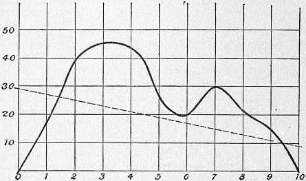
Calibration Curve.

A very neat use of the calibration curve has been made by Professor W.A. Rogers in the automatic correction of screws of dividing machines or lathes. It is possible by the process of grinding, as applied by Rowland, to make a screw which is practically perfect in point of uniformity, but even in this case errors may be introduced by the method of mounting. In the production of divided scales, and more particularly in the case of optical gratings, it is most important that the errors should be as small as possible, and should be automatically corrected during the process of ruling. With this object a scale is ruled on the machine, and the errors of the uncorrected screw are determined by calibrating the scale. A metal template may then be cut out in the form of the calibration-correction curve on a suitable scale. A lever projecting from the nut which feeds the carriage or the slide-rest is made to follow the contour of the template, and to apply the appropriate correction at each point of the travel, by turning the nut through a small angle on the screw. A small periodic error of the screw, recurring regularly at each revolution, may be similarly corrected by means of a suitable cam or eccentric revolving with the screw and actuating the template. This kind of error is important in optical gratings, but is difficult to determine and correct.

Calibration by Comparison with a Standard.—The commonest and most generally useful process of calibration is the direct comparison of the instrument with a standard over the whole range of its scale. It is necessary that the standard itself should have been already calibrated, or else that the law of its indications should be known. A continuous current ammeter, for instance, can be calibrated, so far as the relative values of its readings are concerned, by comparison with a tangent galvanometer, since it is known that the current in this instrument is proportional to the tangent of the angle of deflection. Similarly an alternating current ammeter can be calibrated by comparison with an electrodynamometer, the reading of which varies as the square of the current. But in either case it is neccessary, in order to obtain the readings in amperes, to standardize the instrument for some particular value of the current by comparison with a voltameter, or in some equivalent manner. Whenever possible, ammeters and voltmeters are calibrated by comparison of their readings with those of a potentiometer, the calibration of which can be reduced to the comparison and adjustment of resistances, which is the most accurate of electrical measurements. The commoner kinds of mercury thermometers are generally calibrated and graduated by comparison with a standard. In many cases this is the most convenient or even the only possible method. A mercury thermometer of limited scale reading between 250° and 400° C., with gas under high pressure to prevent the separation of the mercury column, cannot be calibrated on itself, or by comparison with a mercury standard possessing a fundamental interval, on account of difficulties of stem exposure and scale. The only practical method is to compare its readings every few degrees with those of a platinum thermometer under the conditions for which it is to be used. This method has the advantage of combining all the corrections for fundamental interval, &c., with the calibration correction in a single curve, except the correction for variation of zero which must be tested occasionally at some point of the scale.

Authorities.—Mercurial Thermometers: Guillaume, Thermométrie de Précision (Paris, 1889), gives several examples and references to original memoirs. The best examples of comparison and testing of standards are generally to be found in publications of Standards Offices, such as those of the Bureau International des Poids et Mésures at Paris. Dial Resistance-Box: Griffiths, Phil. Trans. A, 1893; Platinum Thermometry-Box: J.A. Harker and P. Chappuis, Phil. Trans. A, 1900; Thomson-Varley Potentiometer and Binary Scale Box: Callendar and Barnes, Phil. Trans. A, 1901.

(H. L. C.)

CALICO, a general name given to plain cotton cloth. The word was spelt in various forms, including “calicut,” which shows its derivation from the Indian city of Calicut or Kolikod, a seaport in the presidency of Madras, and one of the chief ports of intercourse with Europe in the 16th century, where cotton cloths were made. The name seems to have been applied to all kinds of cotton cloths imported from the East. In England it is now applied particularly to grey or bleached cotton cloth used for domestic purposes, and, generally, to any fairly heavy cotton cloth without a pattern. In the United States there is a special application to printed cloth “of a coarser quality than muslin.” In England “printed calico” is a comprehensive term.

CALICUT, a city of British India, in the Malabar district of Madras; on the coast, 6 m. N. of Beypur. In 1901 the population was 76,981, showing an increase of 14% in the decade. The weaving of cotton, for which the place was at one time so famous that its name became identified with its calico, is no longer of any importance. Calicut is of considerable antiquity; and about the 7th century it had its population largely increased by the immigration of the Moplahs, a fanatical race of Mahommedans from Arabia, who entered enthusiastically into commercial life. The Portuguese traveller Pero de Covilham (q.v.) visited Calicut in 1487 and described its possibilities for European trade; and in May 1498 Vasco da Gama, the first European navigator to reach India, arrived at Calicut. At that time it was a very flourishing city, and contained several stately buildings, among which was especially mentioned a Brahminical temple, not inferior to the largest monastery in Portugal. Vasco da Gama tried to establish a factory, but he met with persistent hostility from the local chief (zamorin), and a similar attempt made by Cabral two years later ended in the destruction of the factory by the Moplahs. In revenge the Portuguese bombarded the town, but no further attempt was made for some years to establish a trading settlement there. In 1509 the marshal Don Fernando Coutinho made an unsuccessful attack on the city; and in the following year it was again assailed by Albuquerque with 3000 troops. On this occasion the palace was plundered and the town burnt; but the Portuguese were finally repulsed, and fled to their ships after heavy loss. In the following year they concluded a peace with the zamorin and were allowed to build a fortified factory on the north bank of the Kallayi river, which was however again, and finally, abandoned in 1525. In 1615 the town was visited by an English expedition under Captain Keeling, who concluded a treaty with the zamorin; but it was not until 1664 that an English trading settlement was established by the East India Company. The French settlement, which still exists, was founded in 1698. The town was taken in 1765 by Hyder Ali, who expelled all the merchants and factors, and destroyed the cocoa-nut trees, sandal-wood and pepper vines, that the country reduced to ruin might present no temptation to the cupidity of Europeans. In 1782 the troops of Hyder were driven from Calicut by the British; but in 1788 it was taken and destroyed by his son Tippoo, who carried off the inhabitants to Beypur and treated them with great cruelty. In the latter part of 1790 the country was occupied by the British; and under the treaty concluded in 1792, whereby Tippoo was deprived of half his dominions, Calicut fell to the British. After this event the inhabitants returned and rebuilt the town, which in 1800 consisted of 5000 houses.

As the administrative headquarters of the district, Calicut maintains its historical importance. It is served by the Madras railway, and is the chief seaport on the Malabar coast, and the principal exports are coffee, timber and coco-nut products. There are factories for coffee-cleaning, employing several hundred hands; for coir-pressing and timber-cutting. The town has a cotton-mill, a saw-mill, and tile, coffee and oil works. A detachment of European troops is generally stationed here to overawe the fanatical Moplahs.

CALIFORNIA, one of the Pacific Coast states of the United States of America, physically one of the most remarkable, economically one of the more independent, and in history and social life one of the most interesting of the Union. It is bounded N. by Oregon, E. by Nevada and Arizona, from which last it is separated by the Colorado river, and S. by the Mexican province of Lower California. The length of its medial line N. and S. is about 780 m., its breadth varies from 150 to 350 m., and its total area is 158,207 sq. m., of which 2205 are water surface. In size it ranks second among the states of the Union. The coast is bold and rugged and with very few good harbours; San Diego and San Francisco bays being exceptions. The coast line is more than 1000 m. long. There are eight coast islands, all of inconsiderable size, and none of them as yet in any way important.

Physiography.—The physiography of the state is simple; its main features are few and bold: a mountain fringe along the ocean, another mountain system along the east border, between them—closed in at both ends by their junction—a splendid valley of imperial extent, and outside all this a great area of barren, arid lands, belonging partly to the Great Basin and partly to the Open Basin region.

Along the Pacific, and some 20-40 m. in width, runs the mass of the Coast Range, made up of numerous indistinct chains—most of which have localized individual names—that are broken down into innumerable ridges and spurs, and small valleys drained by short streams of rapid fall. The range is cut by numerous fault lines, some of which betray evidence of recent activity; it is probable that movements along these faults cause the earthquake tremors to which the region is subject, all of which seem to be tectonic. The altitudes of the Coast Range vary from about 2000 to 8000 ft.; in the neighbourhood of San Francisco Bay the culminating peaks are about 4000 ft. in height (Mount Diablo, 3856 ft.; Mount St Helena, 4343 ft.), and to the north and south the elevation of the ranges increases. In the east part of the state is the magnificent Sierra Nevada, a great block of the earth’s crust, faulted along its eastern side and tilted up so as to have a gentle back slope to the west and a steep fault escarpment facing east, the finest mountain system of the United States. The Sierra proper, from Lassen’s Peak to Tehachapi Pass in Kern county, is about 430 m. long (from Mt. Shasta in Siskiyou county to Mt. San Jacinto in Riverside county, more than 600 m.). It narrows to the north and the altitude declines in the same direction. Far higher and grander than the Coast Range, the Sierra is much less complicated, being indeed essentially one chain of great simplicity of structure. It is only here and there that a double line of principal summits exists. The slope is everywhere long and gradual on the west, averaging about 200 ft. to the mile. Precipitous gorges or canyons often from 2000 to 5000 ft. in depth become a more and more marked feature of the range as one proceeds northward; over great portions of it they average probably not more than 20 m. apart. Where the volcanic formations were spread uniformly over the flanks of the mountains, the contrast between the canyons and the plain-like region of gentle slope in which they have been excavated is especially marked and characteristic. The eastern slope is very precipitous, due to a great fault which drops the rocks of the Great Basin region abruptly downward several thousand feet. Rare passes cross the chain, opening at the foot of the mountains on the east and the west high on their flanks, 7000-10,000 ft. above the sea. Between 36° 20′ and 38° the lowest gap of any kind is above 9000 ft., and the average height of those actually used is probably not less than 11,000 ft. The Kearsarge, most used of all, is still higher. Very few in the entire Sierra are passable by vehicles. Some forty peaks are catalogued between 5000 and 8000 ft., and there are eleven above 14,000. The highest portion of the system is between the parallels of 36° 30′ and 37° 30′; here the passes are about 12,000 ft. in elevation, and the peaks range from 13,000 ft. upward, Mount Whitney, 14,502 ft., being the highest summit of the United States, excluding Alaska. From this peak northward there is a gradual decline, until at the point where the Central Pacific crosses in lat. 39° 20′ the elevation is only 7000 ft.

Of the mountain scenery the granite pinnacles and domes of the highest Sierra opposite Owen’s Lake, where there is a drop eastward into the valley of about 10,000 ft. in 10 m.; the snowy volcanic cone of Mt Shasta, rising 10,000 ft. above the adjacent plains; and the lovely valleys of the Coast Range, and the south fork of the King river—all these have their charms; but most beautiful of all is the unique scenery of the Yosemite Valley (q.v.). Much of the ruggedness and beauty of the mountains is due to the erosive action of many alpine glaciers that once existed on the higher summits, and which have left behind their evidences in valleys and amphitheatres with towering walls, polished rock-expanses, glacial lakes and meadows and tumbling waterfalls. Remnants of these glaciers are still to be seen,—as notably on Mt. Shasta,—though shrunk to small dimensions. Glacial action may be studied well as far south as 36°. The canyons are largely the work of rivers, modified by glaciers that ran through them after the rivers had formed them. All of the Sierra lakes and ponds are of glacial origin and there are some thousands of them. The lower lake line is about 8000 ft.; it is lower to the north than to the south, owing to the different climate, and the different period of glacial retrogression. Of these lakes some are fresh, and some—as those of the north-east counties—alkali. The finest of all is Tahoe, 6225 ft. above the sea, lying between the true Sierras and the Basin Ranges, with peaks on several sides rising 4000-5000 ft. above it. It is 1500 ft. deep and its waters are of extraordinary purity (containing only three grains of solid matter to the gallon). Clear Lake, in the Coast Range, is another beautiful sheet of water. It is estimated by John Muir that on an average “perhaps more than a mile” of degradation took place in the last glacial period; but with regard to the whole subject of glacial action in California as in other fields, there is considerable difference of opinion. The same authority counted 65 small residual glaciers between 36° 30′ and 39°; two-thirds of them lie between 37° and 38°, on some of the highest peaks in the district of the San Joaquin, Merced, Tuolumne and Owen’s rivers. They do not descend, on an average, below 11,000 ft.; the largest of all, on Mt. Shasta, descends to 9500 ft. above the sea.

Volcanic action has likewise left abundant traces, especially in the northern half of the range, whereas the evidences of glacial action are most perfect (though not most abundant) in the south. Lava covers most of the northern half of the range, and there are many craters and ash-cones, some recent and of perfect form. Of these the most remarkable is Mt. Shasta. In Owen’s Valley is a fine group of extinct or dormant volcanoes.

Among the other indications of great geological disturbances on the Pacific Coast may also be mentioned the earthquakes to which California like the rest of the coast is liable. From 1850 to 1887 almost 800 were catalogued by Professor E.H. Holden for California, Oregon and Washington. They occur in all seasons, scores of slight tremors being recorded every year by the Weather Bureau; but they are of no importance, and even of these the number affecting any particular locality is small. From 1769 to 1887 there were 10 “destructive” and 24 other “extremely severe” shocks according to the Rossi Forel nomenclatural scale of intensity. In 1812 great destruction was wrought by an earthquake that affected all the southern part of the state; in 1865 the region about San Francisco was violently disturbed; in 1872 the whole Sierra and the state of Nevada were violently shaken; and in 1906 San Francisco (q.v.) was in large part destroyed by a shock that caused great damage elsewhere in the state.

North of 40° N. lat. the Coast Range and Sierra systems unite, forming a country extremely rough. The eastern half of this area is covered chiefly with volcanic plains, very dry and barren, lying between precipitous, although not very lofty, ranges; the western half is magnificently timbered, and toward the coast excessively wet. Between 35° and 36° N. lat. the Sierra at its southern end turns westward toward the coast as the Tehachapi Range. The valley is thus closed to the north and south, and is surrounded by a mountain wall, which is broken down in but a single place, the gap behind the Golden Gate at San Francisco. Through this passes the entire drainage of the interior. The length of the valley is about 450 m., its breadth averages about 40 m. if the lower foothills be included, so that the entire area is about 18,000 sq. m. The drainage basin measured from the water-partings of the enclosing mountains is some three times as great. From the mouth of the Sacramento to Redding, at the northern head of the valley, the rise is 552 ft. in 192 m., and from the mouth of the San Joaquin southward to Kern lake it is 282 ft. in 260 m.

Two great rivers drain this central basin,—the San Joaquin, whose valley comprises more than three-fifths of the entire basin, and the Sacramento, whose valley comprises the remainder. The San Joaquin is a very crooked stream flowing through a low mud-plain, with tule banks; the Sacramento is much less meandering, and its immediate basin, which is of sandy loam, is higher and more attractive than that of the San Joaquin. The eastward flanks of the Coast Range are very scantily forested, and they furnish not a single stream permanent enough to reach either the Sacramento or San Joaquin throughout the dry season. On the eastern side of both rivers are various important tributaries, fed by the more abundant rains and melting snows of the western flank of the Sierra; but these streams also shrink greatly in the dry season. The Feather, emptying into the Sacramento river about 20 m. N. of the city of Sacramento, is the most important tributary of the Sacramento river. A striking feature of the Sacramento system is that for 200 m. north of the Feather it does not receive a single tributary of any importance, though walled in by high mountains. Another peculiar and very general feature of the drainage system of the state is the presence of numerous so-called river “sinks,” where the waters disappear, either directly by evaporation or (as in Death Valley) after flowing for a time beneath the surface. These “sinks” are therefore not the true sinks of limestone regions. The popular name is applied to Owen’s lake, at the end of Owen’s river; to Mono lake, into which flow various streams rising in the Sierra between Mount Dana and Castle Peak; and to Death Valley, which contains the “sink” of the Amargosa river, and evidently was once an extensive lake, although now only a mud-flat in ordinary winters, and a dry, alkaline, desert plain in summer. All these lakes, and the other mountain lakes before referred to, show by the terraces about them that the water stood during the glacial period much higher than it does now. Tulare lake, which with Buena Vista lake and Kern lake receives the drainage of the southern Sierra, shows extreme local variations of shore-line, and is generally believed to have shrunk extremely since 1850, though of this no adequate proof yet exists. In 1900 it was about 200 sq. m. in area. In wet seasons it overflows its banks and becomes greatly extended in area, discharging its surplus waters into the San Joaquin; but in dry seasons the evaporation is so great that there is no such discharge. The drainage of Lassen, Siskiyou and Modoc counties has no outlet to the sea and is collected in a number of great alkaline lakes.

Finally along the sea below Pt. Conception are fertile coastal plains of considerable extent, separated from the interior deserts by various mountain ranges from 5000 to 7000 ft. high, and with peaks much higher (San Bernardino, 11,600; San Jacinto, 10,800; San Antonio, 10,140). Unlike the northern Sierra, the ranges of Southern California are broken down in a number of places. It is over these passes—Soledad, 2822 ft., Cajon, San Gorgonio, 2560 ft.—that the railways cross to the coast. That part of California which lies to the south and east of the southern inosculation of the Coast Range and the Sierra comprises an area of fully 50,000 sq. m., and belongs to the Basin Range region. For the most part it is excessively dry and barren. The Mohave desert—embracing Kern, Los Angeles and San Bernardino, as also a large part of San Diego, Imperial and Riverside counties—belong to the “Great Basin,” while a narrow strip along the Colorado river is in the “Open Basin Region.” They have no drainage to the sea, save fitfully for slight areas through the Colorado river. The Mohave desert is about 2000 ft. above the sea in general altitude. The southern part of the Great Basin region is vaguely designated the Colorado desert. In San Diego, Imperial and Riverside counties a number of creeks or so-called rivers, with beds that are normally dry, flow centrally toward the desert of Salton Sink or “Sea”; this is the lowest part of a large area that is depressed below the level of the sea,—at Salton 263 ft., and 287 ft. at the lowest point. In 1900 the Colorado river (q.v.) was tapped south of the Mexican boundary for water wherewith to irrigate land in the Imperial Valley along the Southern Pacific railway, adjoining Salton Sea. The river enlarged the canal, and finding a steeper gradient than that to its mouth, was diverted into the Colorado desert, flooding Salton Sea;1 and when the break in this river was closed for the second time in February 1907, though much of its water still escaped through minor channels and by seepage, a lake more than 400 sq. m. in area was left. A permanent 60 ft. masonry dam was completed in July 1907. The region to the east of the Sierra, likewise in the Great Basin province, between the crest of that range and the Nevada boundary, is very mountainous. Owen’s river runs through it from north to south for some 180 m. Near Owen’s lake the scenery is extremely grand. The valley here is very narrow, and on either side the mountains rise from 7000 to 10,000 ft. above the lake and river. The Inyo range, on the east, is quite bare of timber, and its summits are only occasionally whitened with snow for a few days during the winter, as almost all precipitation is cut off by the higher ranges to the westward. Still further to the east some 40 m. from the lake is Death Valley (including Lost or Mesquite Valley)—the name a reminder of the fate of a party of “forty-niners” who perished here, by thirst or by starvation and exposure. Death Valley, some 50 m. long and on an average 20-25 m. broad from the crests of the inclosing mountain ranges (or 5-10 m. at their base), constitutes an independent drainage basin. It is below sea level (about 276 ft. according to recent surveys), and altogether is one of the most remarkable physical features of California. The mountains about it are high and bare and brilliant with varied colours. The Amargosa river, entering the valley from Nevada, disappears in the salty basin. Enormous quantities of borax, already exploited, and of nitrate of soda, are known to be present in the surrounding country, the former as almost pure borate of lime in Tertiary lake sediments.

The physiography of the state is the evident determinant of its climate, fauna and flora. California has the highest land and the lowest land of the United States, the greatest variety of temperature and rainfall, and of products of the soil.

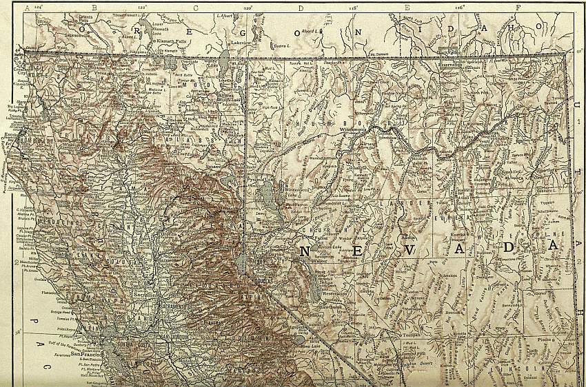
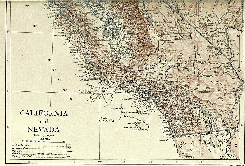
(Click to enlarge top section.) (Click to enlarge bottom section.)

Climate.—The climate is very different from that of the Atlantic coast; and indeed very different from that of any part of the country save that bordering California. Amid great variations of local weather there are some peculiar features that obtain all over the state. In the first place, the climate of the entire Pacific Coast is milder and more uniform in temperature than that of the states in corresponding latitude east of the mountains. Thus we have to go north as far as Sitka in 57° N. lat. to find the same mean yearly temperature as that of Halifax, Nova Scotia, in latitude 44° 39′. And going south along the coast, we find the mean temperature of San Diego 6° or 7° less than that of Vicksburg, Miss., or Charleston, S.C. The quantity of total annual heat supply at Puget Sound exceeds that at Philadelphia, Pittsburg, Cleveland or Omaha, all more than 500 m. farther south; Cape Flattery, exposed the year round to cold ocean fogs, receives more heat than Eastport, Maine, which is 3° farther south and has a warmer summer. In the second place, the means of winter and summer are much nearer the mean of the year in California than in the east. This condition of things is not so marked as one goes inward from the coast; yet everywhere save in the high mountains the winters are comparatively mild. In the third place, the division of the year into two seasons—a wet one and a dry (and extremely dusty) one—marks this portion of the Pacific Coast in the most decided manner, and this natural climatic area coincides almost exactly in its extension with that of California; being truly characteristic neither of Lower California nor of the greater part of Oregon, though more so of Nevada and Arizona. And finally, in the fourth place, except on the coast the disagreeableness of the heat of summer is greatly lessened by the dryness of the air and the consequent rapidity of evaporation. Among the peculiarities of Californian climate it is not one of the least striking that as one leaves the Sacramento or San Joaquin plains and travels into the mountains it becomes warmer, at least for the first 2000 or 3000 ft. of ascent.

Along both the Coast Range and the Sierra considerable rainfall is certain, although, owing to the slight snow accumulations of the former, its streams are decidedly variable. A heavy rain-belt, with a normal fall of more than 40 in., covers all the northern half of the Sierra and the north-west counties; shading off from this is the region of 10-20 in. fall, which covers all the rest of the state save Inyo, Kern and San Bernardino counties, Imperial county and the eastern portion of Riverside county; the precipitation of this belt is from 0 to 10 in. In excessively dry years the limits of this last division may include all of the state below Fresno and the entire Central Valley as well. In the mountains the precipitation increases with the altitude; above 6000 or 7000 ft. it is almost wholly in the form of snow; and this snow, melting in summer, is of immense importance to the state, supplying water once for placer mining and now for irrigation. The north-west counties are extremely wet; many localities here have normal rainfalls of 60-70 in. and even higher annually, while in extreme seasons as much as 125 in. falls. Along the entire Pacific Coast, but particularly N. of San Francisco, there is a night fog from May to September. It extends but a few miles inland, but within this belt is virtually a prolongation of the rainy season and has a marked effect on vegetation. Below San Francisco the precipitation decreases along the coast, until at San Diego it is only about 10 in. The south-east counties are the driest portions of the United States. At Ogilby, Volcano, Indio and other stations on the Southern Pacific line the normal annual precipitation is from 1.5 to 2.5 in.; and there are localities near Owen’s lake, even on its very edge, that are almost dry. For days in succession when it storms along the Southern California coasts and dense rain clouds blow landwards to the mountains, leaving snow or rain on their summits, it has been observed that within a few miles beyond the ridge the contact of the desert air dissipates the remaining moisture of the clouds into light misty masses, like a steam escape in cold air. The extreme heat of the south-east is tempered by the extremely low humidity characteristic of the Great Basin, which in the interior of the two southernmost counties is very low. The humidity of places such as Fresno, Sacramento and Red Bluff in the valley varies from 48 to 58. Many places in northern, southern, central, mountain and southern coastal California normally have more than 200 perfectly clear days in a year; and many in the mountains and in the south, even on the coast, have more than 250. The extreme variability in the amount of rainfall is remarkable.2 The effects of a season of drought on the dry portions of the state need not be adverted to; and as there is no rain or snow of any consequence on the mountains during summer, a succession of dry seasons may almost bare the ranges of the accumulated stock of previous winter snows, thus making worse what is already bad.

The Colorado desert (together with the lower Gila Valley of Arizona) is the hottest part of the United States. Along the line of the Southern Pacific the yearly extreme is frequently from 124° to 129° F. (i.e. in the shade, which is almost if not quite the greatest heat ever actually recorded in any part of the world). At the other extreme, temperatures of -20° to -36° are recorded yearly on the Central (Southern) Pacific line near Lake Tahoe. The normal annual means of the coldest localities of the state are from 37° to 44° F.; the monthly means from 20° to 65° F. The normal annual means on Indio, Mammoth Tanks, Salton and Volcano Springs are from 73.9° to 78.4 F.; the monthly means from 52.8° to 101.3° (frequently 95° to 98°). The normal trend of the annual isotherms of the state is very simple: a low line of about 40° circles the angle in the Nevada boundary line; 50° normally follows the northern Sierra across the Oregon border; lines of higher temperature enclose the Great Valley; and lines of still higher temperature—usually 60° to 70°, in hotter years 60° to 75°—run transversely across the southern quarter of the state.

Another weather factor is the winds, which are extremely regular in their movements. There are brisk diurnal sea-breezes, and seasonal trades and counter-trades. Along the coast an on-shore breeze blows every summer day; in the evening it is replaced by a night-fog, and the cooler air draws down the mountain sides in opposition to its movement during the day. In the upper air a dry off-shore wind from the Rocky Mountain plateau prevails throughout the summer; and in winter an on-shore rain wind. The last is the counter-trade, the all-year wind of Alaska and Oregon; it prevails in winter even off Southern California.

There is the widest and most startling variety of local climates. At Truckee, for example, lying about 5800 ft. above the sea near Lake Tahoe, the lowest temperature of the year may be -25° F. or colder, when 70 m. westward at Rocklin, which lies in the foothills about 250 ft. above the sea, the mercury does not fall below 28°. Snow never falls at Rocklin, but falls in large quantity at Truckee; ice is the crop of the one, oranges of the other, at the same time. There are points in Southern California where one may actually look from sea to desert and from snow to orange groves. Distance from the ocean, situation with reference to the mountain ranges, and altitude are all important determinants of these climatic differences; but of these the last seems to be most important. At any rate it may be said that generally speaking the maximum, minimum and mean temperatures of points of approximately equal altitude are respectively but slightly different in northern or southern California.3

Death Valley surpasses for combined heat and aridity any meteorological stations on earth where regular observations are taken, although for extremes of heat it is exceeded by places in the Colorado desert. The minimum daily temperature in summer is rarely below 70° F. and often above 90° F. (in the shade), while the maximum may for days in succession be as high as 120° F. A record of 6 months (1891) showed an average daily relative humidity of 30.6 in the morning and 15.6 in the evening, and the humidity sometimes falls to 5. Yet the surrounding country is not devoid of vegetation. The hills are very fertile when irrigated, and the wet season develops a variety of perennial herbs, shrubs and annuals.

Fauna.—California embraces areas of every life-zone of North America: of the boreal, the Hudsonian and Canadian subzones; of the transition, the humid Pacific subzone; of the upper austral, the arid or upper Sonoran subzone; of the lower austral, the arid or lower Sonoran; of the tropical, the “dilute arid” subzone. As will be inferred from the above account of temperature, summer is longer in the north, and localities in the Valley have more hours of heat than do those of south California. Hence that climatic characteristic of the entire Pacific Coast—already referred to and which is of extreme importance in determining the life-zones of California—the great amount of total annual heat supply at comparatively high latitudes. A low summer temperature enables northern species to push far southward, while the high heat total of the year enables southern species to push far north. The resultant intermingling of forms is very marked and characteristic of the Pacific Coast states. The distribution of life-zones is primarily a matter of altitude and corresponds to that of the isotherms. The mountain goat and mountain sheep live in the Sierran upper-land, though long ago well-nigh exterminated. The Douglas red squirrel is ubiquitous in the Sierran forests and their most conspicuous inhabitant. White-tailed deer and especially black-tails are found on the high Sierra; the mule deer, too, although its habitat is now mainly east of the range, on the plateau, is also met with. Grizzly, black, cinnamon and brown bears are all Californian species once common and to-day rare. When Americans began to rule in California elk and antelope herded in great numbers in the Great Valley; the former may to-day sometimes be seen, possibly, in the northern forests, and the latter occasionally cross into the state from Nevada. The sage-hen is abundant on the eastern flank of the Sierra. Grouse, quail, crows and woodpeckers (Melanerpes formicivorus) furnish species characteristic of the state. There are various species of ground-squirrels and gophers, which are very abundant. Noteworthy in the animal life of the lower Sonoran and tropic region are a variety of snakes and lizards, desert rats and mice; and, among birds, the cactus wren, desert thrasher, desert sparrow, Texas night-hawk, mocking-bird and ground cuckoo or road runner (Geococcyx Californianus). The California vulture, the largest flying bird in North America and fully as large as the Andean condor, is not limited to California but is fairly common there. In the zoology and botany of California as of the rest of the Pacific Coast, the distinctions between the upper austral and humid transition zones are largely obliterated; and as one passes southward into the arid lands, life forms of both these zones intermingle with those of the arid transition.

Fish are abundant. The United States fish commission, and an active state commission established in 1869, have done much to preserve and increase this source of food. In 1904 the yield of the fisheries of the three Pacific Coast states was 168,600,000 lbs, valued at $6,681,000,—nearly half that of the New England states, more than one-third that of the Middle Atlantic states and more than that of the South Atlantic and Gulf states combined. Of the total, California yielded between a quarter and a third. A third of her fish comes from the Sacramento river. Some 230—more or less—marine food fishes are to be found in the market at San Francisco. The exports of fish from that port from 1892-1899 were valued at from $2,000,000 to $2,500,000 annually. Native oysters are small and of peculiar flavour; eastern varieties also are fattened, but not bred in California waters. Shrimp are abundant; the shrimp fishers are Chinese and four-fifths of the catch is exported to China. Sturgeon were once the cheapest fish after salmon; to-day, despite all efforts to increase the supply, they are the dearest. Salmon, once threatened with extinction, have been saved, maintained in good supply, and indeed have probably regained their pristine abundance. Shad and striped bass are both very abundant and cheap. Black bass, flounders, terrapin, sea-turtles, perch, turbot, sole and catfish are also common. Great herds of seals once lay like toll-gatherers off the Golden Gate and other bays of the coast, taking a large share of the salmon and other fish; but they are no longer common. The sea-lions sometimes raid the rivers for 100 m. inland. They have greatly increased since hunting them for their hides and oil ceased to be profitable, and thousands sometimes gather on the Farallones, off the Golden Gate.

Flora.—Inclusiveness of range in the distribution of vegetable life is perhaps more suggestive than the distribution of animal species. The variation is from dwarf mountain pine to giant cactus and dates. The humid transition belt is the habitat of California’s magnificent forests. Nut pine, juniper and true sage-brush (Artemisia tridentata) characterize the upper Sonoran,—although the latter grows equally in the transition zone. Cereals, orchard fruits and alfalfa are of primary importance in the upper and of secondary importance in the lower Sonoran. In the arid portions of this and the tropic areas the indigenous plants are creosote, mesquite and alfileria bushes, desert acacias, paloverdes, alkali-heath, salt grass, agaves, yuccas (especially the Spanish-bayonet and Joshua tree) and cactuses. Among exotics the Australian saltbush spreads successfully over the worst alkali land. The introduction of other exotics into these zones,—made humid by irrigation, which converts them, the one into true austro-riparian the other into true humid tropical,—has revolutionized the agricultural, and indeed the whole, economy of California. At the two ends of Cajon Pass, only four or five kilometres apart, are the two utterly distinct floras of the Mohave desert and the San Bernardino valley. Despite the presence of the pass, plants do not spread, so great is the difference of climatic conditions. On the desert the same plant will vary in different years from 4 in. to 10 ft. in height when equally mature, according to the rainfall and other conditions of growth. Many mature plants are not taller than 0.4 to 0.8 in. The tree yucca often attains a height of 20 to 25 ft., and a diameter of 1.5 ft. About 600 species of plants were catalogued in desert California in 1891 by a government botanical party. The flora of the coast islands of California is very interesting. On Santa Cruz Professor Joseph Le Conte found 248 species, nearly all of which are distinctively Californian, 48 being peculiar to the surrounding islands and 28 peculiar to Southern California. Various other things indicate a separation of the islands from the mainland in quaternary times; since which, owing to the later southward movement on the continent of northern forms in glacial times, there has been a struggle for existence on the mainland from which the islands have largely escaped.

Forests.—The forests and agricultural crops of the state demand particular notice. In 1900 the woodland was estimated by the United States census at 22% of the state’s area, and the total stand at 200,000 million ft. of timber. The variety of forest trees is not great, but some of the California trees are unique, and the forests of the state are, with those of Oregon and Washington, perhaps the most magnificent of the world. At least the coniferous forests which make up nine-tenths of California’s woodland surpass all others known in number of species and in the size and beauty of the trees. Forty-six species occur, namely, 32 species of pitch trees (18 pines), 12 species of the cypresses and their allies (2 sequoia), and 2 species of yews or their allies. Peculiar to California are the two species of sequoia (q.v.),—the redwood (S. sempervirens), and the big-tree (S. gigantea), remnants of an earlier age when they were common in other parts of the world. The redwood grows only in a narrow strip on the Coast Range from Southern Oregon (where there are not more than 1000 acres) down nearly to the Golden Gate, in a habitat of heavy rains and heavy fogs. They cover an area of about 2000 sq. m. almost unmixed with other species. One fine grove stands S. of San Francisco near Santa Cruz. These noble trees attain very often a height of more than 300 ft., frequently of 350 and even more, and a butt diameter of more than 15 to 20 ft., with clean, straight fluted trunks rising 200 ft. below the lowest branches. They grow in a very dense timber stand; single acres have yielded 1,500,000 ft. B.M. of lumber, and single trees have cut as high as 100,000 ft. The total stand in 1900 was estimated by the United States census as 75,000,000,000 ft., and the ordinary stand per acre varies from 25,000 to 150,000 ft., averaging probably 60,000 ft. The redwood is being rapidly used for lumber. There is nowhere any considerable young growth from seed, although this mode of reproduction is not (as often stated) unknown; the tree will reproduce itself more than once from the stump (hence its name). In thirty years a tree has been known to grow to a height of 80 ft. and a diameter of 16 in. The wood contains no pitch and much water, and in a green condition will not burn. To this fact it owes its immunity from the forest fires which wreak frightful havoc among the surrounding forests. As the redwood is limited to the Coast Range, so the big tree is limited wholly to the Sierra Nevada. Unlike the redwood the big tree occurs in scattered groves (ten in all) among other species. Its habitat extends some 200 m., from latitude 36° to 39°, nowhere descending much below an altitude of 5000 ft., nor rising above 8000 ft. The most northerly grove and the nearest to San Francisco is the Calaveras Grove near Stockton; the Mariposa Grove just south of the Yosemite National Park, is a state reservation and easily accessible to tourists. The noblest groves are near Visalia, and are held as a national park. The average height is about 275 ft., and the diameter near the ground 20 ft.; various individuals stand over 300 ft., and a diameter of 25 ft. is not rare. One tree measures 35.7 ft. inside the bark 4 ft. above the ground, 10 ft. at 200 ft. above the ground, and is 325 ft. tall. Specimens have been cut down that were estimated to be 1300 and even 2200 years old; many trees standing are presumably 2500 years old. It is the opinion of John Muir that the big tree would normally live 5000 years or more; that the California groves are still in their prime; that, contrary to general ideas, the big tree was never more widely distributed than now, at least not within the past 8000 or 10,000 years; that it is not a decaying species, but that on the contrary “no tree of all the forest is more enduringly established in concord with climate and soil,” growing like the mountain pine even on granite, and in little danger save from the greed of the lumberman; but other excellent authorities consider it as hardly holding its own, especially in the north. Three main wood belts cover the flanks of the Sierra: the lower or main pine belt, the silver fir belt, and the upper pine belt. The sugar pine, the yellow or silver pine and the Douglas spruce (considerably smaller than in Oregon and Washington), are rivals in stature and nobility, all attaining 200 ft. or more when full grown; and the incense cedar reaches a height of 150 ft. In this belt and the following one of firs the big tree also grows. The white silver fir (abies concolor) and the silver or red fir (ab. magnifica), standing 200 to 250 ft., make up almost wholly the main forest belt from 5000 to 9000 ft. for some 450 m. Above the firs come the tamarack, constituting the bulk of the lower Alpine forest; the hardy long-lived mountain pine; the red cedar or juniper, growing even on the baldest rocks; the beautiful hemlock spruce; the still higher white pine, nut pine, needle pine; and finally, at 10,000 to 12,000 ft., the dwarf pine, which grows in a tangle on the earth over which one walks, and may not show for a century’s growth more than a foot of height or an inch of girth. The Nevada slope of the mountains below 7500 ft. is covered with the nut pine down to the sage plains. Its nuts are gathered in enormous amounts by the Indians for food; and it is estimated that the yearly harvest of these nuts exceeds in bulk that of all the cereals of California (John Muir). On the Sierra the underbrush is characterized by the pungent manzanita, the California buckeye and the chamiso; the last two growing equally abundantly on the Coast Range. The chamiso and the manzanita, with a variety of shrubby oaks and thorny plants, often grow together in a dense and sometimes quite impenetrable undergrowth, forming what is known as “chaparral”; if the chamiso occurs alone the thicket is a “chamisal.” The elm, the hickory, the beech, the chestnut, and many others of the most characteristic and useful trees of the eastern states were originally entirely wanting in California. Oaks are abundant; they are especially characteristic of the Great Valley, where they grow in magnificent groves. Up to 1910 national forest reserves amounted to 27,968,510 acres. In 1909 Congress created a national forest to include the big tree groves in Calaveras and Tuolumne counties. One of the noblest redwood areas (that of Santa Cruz county) is a state reservation (created in 1901). Even within reservations almost all the merchantable timber is owned by private individuals. In addition to native trees many others—especially ornamental species—have been successfully introduced from various parts of the world.

Soil.—Sand and loams in great variety, grading from mere sand to adobe, make up the soils of the state. The plains of the north-east counties are volcanic, and those of the south-east sandy. It is impossible to say with accuracy what part of the state may properly be classed as tillable. The total farm acreage in 1900 was 28,828,951 acres, of which 41.5% were improved; since 1880 the absolute amount of improved land has remained practically constant, despite the extraordinary progress of the state in these years. Much land is too rough, too elevated or too arid ever to be made agriculturally available; but irrigation, and the work of the state and national agricultural bureaus in introducing new plants and promoting scientific farming, have accomplished much that once seemed impossible. The peculiarities of the climate, especially its division into two seasons, make Californian (and Southern Arizona) agriculture very different from that of the rest of the country. During the winter no shelter is necessary for live-stock, nor, during summer, for the grains that are harvested in June and July, and may lie for weeks or months in the field. The mild, wet winter is the season of planting and growth, and so throughout the year there is a succession of crops. The dangers of drought in the long dry seasons particularly increase the uncertainties of agriculture in regions naturally arid. Irrigation was introduced in Southern California before 1780, but its use was desultory and its spread slow till after 1850. In 1900 almost 1,500,000 acres were irrigated—an increase of 46% since 1890. About half of this total was in San Joaquin Valley. California has the greatest area of irrigated land of any state in the Union, and offers the most complete utilization of resources. In the south artesian wells, and in the Great Valley the rivers of the Sierra slope, are the main source of water-supply. On nearly all lands irrigated some crops will grow in ordinary seasons without irrigation, but it is this that makes possible selection of crops; practically indispensable for all field and orchard culture in the south, save for a few moist coastal areas, it everywhere increases the yield of all crops and is practised generally all over the state. Of the acreage devoted to alfalfa in 1899, 76.2% was irrigated; of that devoted to subtropical fruits, 71.7%. Small fruits, orchard fruits, hay, garden products and grains are decreasingly dependent on irrigation; wheat, which was once California’s great staple, is (for good, but not for best results) comparatively independent of it,—hence its early predominance in Californian agriculture, due to this success on arid lands since taken over for more remunerative irrigated crops.