VOLUME II SLICE VIII Atherstone to Austria (continued 2)

The Atlantic is by far the saltest of the great oceans. Its saltest waters are found at the surface in two belts, one extending east and west in the North Atlantic between 20° and 30° N. lat., and another of almost equal salinity Salinity. extending eastwards from the coast of South America in 10° to 20° S. lat. In the equatorial region between these belts the salinity is markedly less, especially in the eastern part. North of the North Atlantic maximum the waters become steadily fresher as latitude increases until the channels opening into the Arctic basin are reached. In all of these water of relatively high salinity usually appears for a long distance towards the north on the eastern side of the channel, while on the western side the water is comparatively fresh; but great variations occur at different seasons and in different years. In the higher latitudes of the South Atlantic the salinity diminishes steadily and tends to be uniform from east to west, except near the southern extremity of South America, where the surface waters are very fresh. Our knowledge of the salinity of waters below the surface is as yet very defective, large areas being still unrepresented by a single observation. The chief facts already established are the greater saltness of the North Atlantic compared with the South Atlantic at all depths, and the low salinity at all depths in the eastern equatorial region, off the Gulf of Guinea.

The wind circulation over the Atlantic is of a very definite character. In the South Atlantic the narrow land surfaces of Africa and South America produce comparatively little effect in disturbing the normal planetary circulation. Meteorology. The tropical belt of high atmospheric pressure is very marked in winter; it is weaker during the summer months, and at that season the greater relative fall of pressure over the land cuts it off into an oval-shaped anticyclone, the centre of which rests on the coolest part of the sea surface in that latitude, near the Gulf of Guinea. South of this anticyclone, from about the latitude of the Cape, we find the region where, on account of the uninterrupted sea surface right round the globe, the planetary circulation is developed to the greatest extent known; the pressure gradient is steep, and the region is swept continuously by strong westerly winds—the “roaring forties.”

In the North Atlantic the distribution of pressure and resulting wind circulation are very largely modified by the enormous areas of land and frozen sea which surround the ocean on three sides. The tropical belt of high pressure persists all the year round, but the immense demand for air to supply the ascending currents over the heated land surfaces in summer causes the normal descending movement to be largely reinforced; hence the “North Atlantic anticyclone” is much larger, and its circulation more vigorous, in summer than in winter. Again, during the winter months pressure is relatively high over North America, Western Eurasia and the Arctic regions; hence vast quantities of air are brought down to the surface, and circulation must be kept up by ascending currents over the ocean. The Atlantic anticyclone is, therefore, at its weakest in winter, and on its polar side the polar eddy becomes a trough of low pressure, extending roughly from Labrador to Iceland and Jan Mayen, and traversed by a constant succession of cyclones. The net effect of the surrounding land is, in fact, to reverse the seasonal variations of the planetary circulation, but without destroying its type. In the intermediate belt between the two high-pressure areas the meteorological equator remains permanently north of the geographical equator, moving between it and about 11° N. lat.

The part of this atmospheric circulation which is steadiest in its action is the trade winds, and this is, therefore, the most effective in producing drift movement of the surface waters. The trade winds give rise, in the region most exposed to their influence, to two westward-moving drifts—the equatorial currents, which are separated in parts of their course by currents moving in the opposite direction along the equatorial belt. These last may be of the nature of “reaction” currents; they are collectively known as the equatorial counter-current. On reaching the South American coast, the southern equatorial current splits into two parts at Cape St Roque: one branch, Currents. the Brazil current, is deflected southwards and follows the coast as a true stream current at least as far as the river Plate. The second branch proceeds north-westwards towards the West Indies, where it mingles with the waters of the northern equatorial; and the two drifts, blocked by the <-shape of the land, raise the level of the surface in the Gulf of Mexico, the Caribbean Sea, and in the whole area outside the West Indies. This congestion is relieved by what is probably the most rapid and most voluminous stream current in the world, the Gulf Stream, which runs along the coast of North America, separated from it by a narrow strip of cold water, the “cold wall,” to a point off the south-east of Newfoundland. At this point the Gulf Stream water mixes with that from the Labrador current (see below), and a drift current eastwards is set up under the influence of the prevailing westerly winds: this is generally called the Gulf Stream drift. When the Gulf Stream drift approaches the eastern side of the Atlantic it splits into two parts, one going southwards along the north-west coast of Africa, the Canaries current, and another turning northwards and passing to the west of the British Isles. Most of the Canaries current re-enters the northern equatorial, but a certain proportion keeps to the African coast, unites with the equatorial return currents, and penetrates into the Gulf of Guinea. This last feature of the circulation is still somewhat obscure; it is probably to be accounted for by the fact that on this part of the coast the prevailing winds, although to a considerable extent monsoonal, are off-shore winds, blowing the surface waters out to sea, and the place of the water thus removed is filled up by the water derived either from lower levels or from “reaction” currents.

The movements of the northern branch of the Gulf Stream drift have been the object of more careful and more extended study than all the other currents of the ocean put together, except, perhaps, the Gulf Stream itself. The cruises of the “Porcupine” and “Lightning” which led directly to the despatch of the “Challenger” expedition, were altogether within its “sphere of influence”; so also was the great Norwegian Atlantic expedition. More recently, the area has been further explored by the German expedition in the ss. “National,” the Danish “Ingolf” expedition, and the minor expeditions of the “Michael Sars,” “Jackal,” “Research,” &c., and since 1902 it has been periodically examined by the International Council for the Study of the Sea. Much has also been done by the discussion of observations made on board vessels belonging to the mercantile marine of various countries. It may now be taken as generally admitted that the current referred to breaks into three main branches. The first passes northwards, most of it between the Faeroe and Shetland Islands, to the coast of Norway, and so on to the Arctic basin, which, as Nansen has shown, it fills to a great depth. The second, the Irminger stream, passes up the west side of Iceland; and the third goes up to the Greenland side of Davis Strait to Baffin Bay. These branches are separated from one another at the surface by currents moving southwards: one passes east of Iceland; the second, the Greenland current, skirts the east coast of Greenland; and the third, the Labrador current already mentioned, follows the western side of Davis Strait.

The development of the equatorial and the Brazil currents in the South Atlantic has already been described. On the polar side of the high-pressure area a west wind drift is under the control of the “roaring forties,” and on reaching South Africa part of this is deflected and sent northwards along the west coast as the cold Benguella current which rejoins the equatorial. In the central parts of the two high-pressure areas there is practically no surface circulation. In the North Atlantic this region is covered by enormous banks of gulf-weed (Sargassum bucciferum), hence the name Sargasso Sea. The Sargasso Sea is bounded, roughly, by the lines of 20°-35° N. lat. and 40°-75° W. long.

The sub-surface circulation in the Atlantic may be regarded as consisting of two parts. Where surface water is banked up against the land, as by the equatorial and Gulf Stream drift currents, it appears to penetrate to very considerable depths; the escaping stream currents are at first of great vertical thickness and part of the water at their sources has a downward movement. In the case of the Gulf Stream, which is not much impeded by the land, this descending motion is relatively slight, being perhaps largely due to the greater specific gravity of the water; it ceases to be perceptible beyond about 500 fathoms. On the European-African side the descending movement is more marked, partly because the coast-line is much more irregular and the northward current is deflected against it by the earth’s rotation, and partly because of the outflow of salt water from the Mediterranean; here the movement is traceable to at least 1000 fathoms. The northward movement of water across the Norwegian Sea extends down from the surface to the Iceland-Shetland ridge, where it is sharply cut off; the lower levels of the Norwegian Sea are filled with ice-cold Arctic water, close down to the ridge. The south-moving currents originating from melting ice are probably quite shallow. The second part of the circulation in the depth is the slow “creep” of water of very low temperature along the bottom. The North Atlantic being altogether cut off from the Arctic regions, and the vertical circulation being active, this movement is here practically non-existent; but in the South Atlantic, where communication with the Southern Ocean is perfectly open, Antarctic water can be traced to the equator and even beyond.

The tides of the Atlantic Ocean are of great complexity. The tidal wave of the Southern Ocean, which sweeps uninterruptedly round the globe from the east to west, generates a secondary wave between Africa and South America, which travels north at a rate dependent only on the depth of the ocean. With this “free” wave is combined a “forced” wave, generated, by the direct action of the sun and moon, within the Atlantic area itself. Nothing is known about the relative importance of these two waves.

(H. N. D.)

See also Oceans and Oceanography.

ATLANTIS, Atlantis, or Atlantica, a legendary island in the Atlantic Ocean, first mentioned by Plato in the Timaeus. Plato describes how certain Egyptian priests, in a conversation with Solon, represented the island as a country larger than Asia Minor and Libya united, and situated just beyond the Pillars of Hercules (Straits of Gibraltar). Beyond it lay an archipelago of lesser islands. According to the priests, Atlantis had been a powerful kingdom nine thousand years before the birth of Solon, and its armies had overrun the lands which bordered the Mediterranean. Athens alone had withstood them with success. Finally the sea had overwhelmed Atlantis, and had thenceforward become unnavigable owing to the shoals which marked the spot. In the Critias Plato adds a history of the ideal commonwealth of Atlantis. It is impossible to decide how far this legend is due to Plato’s invention, and how far it is based on facts of which no record remains. Medieval writers, for whom the tale was preserved by the Arabian geographers, believed it true, and were fortified in their belief by numerous traditions of islands in the western sea, which offered various points of resemblance to Atlantis. Such in particular were the Greek Isles of the Blest, or Fortunate Islands, the Welsh Avalon, the Portuguese Antilia or Isle of Seven Cities, and St Brendan’s island, the subject of many sagas in many languages. These, which are described in separate articles, helped to maintain the tradition of an earthly paradise which had become associated with the myth of Atlantis; and all except Avalon were marked in maps of the 14th and 15th centuries, and formed the object of voyages of discovery, in one case (St Brendan’s island) until the 18th century. In early legends, of whatever nationality, they are almost invariably described in terms which closely resemble Homer’s account of the island of the Phaeacians (Od. viii.)—a fact which may be an indication of their common origin in some folk-tale current among several races. Somewhat similar legends are those of the island of Brazil (q.v.), of Lyonnesse (q.v.), the sunken land off the Cornish coast, of the lost Breton city of Is, and of Mayda or Asmaide—the French Isle Verte and Portuguese Ilha Verde or “Green Island”—which appears in many folk-tales from Gibraltar to the Hebrides, and until 1853 was marked on English charts as a rock in 44° 48′ N. and 26° 10′ W. After the Renaissance, with its renewal of interest in Platonic studies, numerous attempts were made to rationalize the myth of Atlantis. The island was variously identified with America, Scandinavia, the Canaries and even Palestine; ethnologists saw in its inhabitants the ancestors of the Guanchos, the Basques or the ancient Italians; and even in the 17th and 18th centuries the credibility of the whole legend was seriously debated, and sometimes admitted, even by Montaigne, Buffon and Voltaire.

For the theory that Atlantis is to be identified with Crete in the Minoan period, see “The Lost Continent” in The Times (London) for the 19th of February 1909. See also “Dissertation sur l’Atlantide” in T.H. Martin’s Études sur le Timée (1841).

ATLAS, in Greek mythology, the “endurer,” a son of the Titan Iapetus and Clymene (or Asia), brother of Prometheus. Homer, in the Odyssey (i. 52) speaks of him as “one who knows the depths of the whole sea, and keeps the tall pillars which hold heaven and earth asunder.” In the first instance he seems to have been a marine creation. The pillars which he supported were thought to rest in the sea, immediately beyond the most western horizon. But as the Greeks’ knowledge of the west increased, the name of Atlas was transferred to a hill in the north-west of Africa. Later, he was represented as a king of that district, rich in flocks and herds, and owner of the garden of the Hesperides, who was turned into a rocky mountain when Perseus, to punish him for his inhospitality, showed him the Gorgon’s head (Ovid, Metam. iv. 627). Finally, Atlas was explained as the name of a primitive astronomer, who was said to have made the first celestial globe (Diodorus iii. 60). He was the father of the Pleiades and Hyades; according to Homer, of Calypso. In works of art he is represented as carrying the heavens or the terrestrial globe. The Farnese statue of Atlas in the Naples museum is well known.

The plural form Atlantes is the classical term in architecture for the male sculptured figures supporting a superstructure as in the baths at Pompeii, and in the temple at Agrigentum in Sicily. In 18th-century architecture half-figures of men with strong muscular development were used to support balconies (see Caryatides and Telamones).

A figure of Atlas supporting the heavens is often found as a frontispiece in early collections of maps, and is said to have been first thus used by Mercator. The name is hence applied to a volume of maps (see Map), and similarly to a volume which contains a tabular conspectus of a subject, such as an atlas of ethnographical, subjects or anatomical plates. It is also used of a large size of drawing paper.

The name “atlas,” an Arabic word meaning “smooth,” applied to a smooth cloth, is sometimes found in English, and is the usual German word, for “satin.”

ATLAS MOUNTAINS, the general name for the mountain chains running more or less parallel to the coast of North-west Africa. They extend from Cape Nun on the west to the Gulf of Gabes on the east, a distance of some 1500 m., traversing Morocco, Algeria and Tunisia. To their south lies the Saharan desert. The Atlas consist of many distinct ranges, but they can be roughly divided into two main chains: (1) the Maritime Atlas, i.e. the ranges overlooking the Mediterranean from Ceuta to Cape Bon; (2) the inner and more elevated ranges, which, starting from the Atlantic at Cape Ghir in Sús, run south of the coast ranges and are separated from them by high plateaus. This general disposition is seen most distinctly in eastern Morocco and Algeria. The western inner ranges are the most important of the whole system, and in the present article are described first as the Moroccan Ranges. The maritime Atlas and the inner ranges in Algeria and Tunisia are then treated under the heading Eastern Ranges.

The Moroccan Ranges.—This section of the Atlas, known to the inhabitants of Morocco by its Berber name, Idráren Dráren or the “Mountains of Mountains,” consists of five distinct ranges, varying in length and height, but disposed more or less parallel to one another in a general direction from south-west to north-east, with a slight curvature towards the Sahara.

1. The main range, that known as the Great Atlas, occupies a central position in the system, and is by far the longest and loftiest chain. It has an average height of over 11,000 ft., whereas the loftiest peaks in Algeria do not exceed 8000 ft., and the highest in Tunisia are under 6000 ft. Towards the Dahra district at the north-east end the fall is gradual and continuous, but at the opposite extremity facing the Atlantic between Agadir and Mogador it is precipitous. Although only one or two peaks reach the line of perpetual snow, several of the loftiest summits are snowclad during the greater part of the year. The northern sides and tops of the lower heights are often covered with dense forests of oak, cork, pine, cedar and other trees, with walnuts up to the limit of irrigation. Their slopes enclose well-watered valleys of great fertility, in which the Berber tribes cultivate tiny irrigated fields, their houses clinging to the hill-sides. The southern flanks, being exposed to the hot dry winds of the Sahara, are generally destitute of vegetation.

At several points the crest of the range has been deeply eroded by old glaciers and running waters, and thus have been formed a number of devious passes. The central section, culminating in Tizi n ’Tagharat or Tinzár, a peak estimated at 15,000 ft. high, maintains a mean altitude of 11,600 ft., and from this great mass of schists and sandstones a number of secondary ridges radiate in all directions, forming divides between the rivers Dra’a, Sús, Um-er-Rabíā, Sebú, Mulwíya and Ghír, which flow respectively to the south-west, the west, north-west, north, north-east and south-east. All are swift and unnavigable, save perhaps for a few miles from their mouths. With the exception of the Dra’a, the streams rising on the side of the range facing the Sahara do not reach the sea, but form marshes or lagoons at one season, and at another are lost in the dry soil of the desert.

For a distance of 100 m. the central section nowhere presents any passes accessible to caravans, but south-westward two gaps in the range afford communication between the Tansíft and Sús basins, those respectively of Gindáfi and Bíbáwan. A few summits in the extreme south-west in the neighbourhood of Cape Ghir still exceed 11,000 ft., and although the steadily rising ground from the coast and the prominence of nearer summits detract from the apparent height, this is on an average greater than that of the European Alps. The most imposing view is to be obtained from the plain of Marrákesh, only some 1000 ft. above sea-level, immediately north of the highest peaks. Besides huge masses of old schists and sandstones, the range contains extensive limestone, marble, diorite, basalt and porphyry formations, while granite prevails on its southern slopes. The presence of enormous glaciers in the Ice Age is attested by the moraines at the Atlantic end, and by other indications farther east. The best-known passes are: (1) The Bíbáwan in the upper Wad Sús basin (4150 ft.); (2) the Gindáfi, giving access from Marrákesh to Tárudánt, rugged and difficult, but low; (3) the Tagharat, difficult and little used, leading to the Dra’a valley (11,484 ft.); (4) the Gláwi (7600 ft.); (5) Tizi n ’Tilghemt (7250 ft.), leading to Tafilet (Tafílált) and the Wad Ghír.

2. The lower portion of the Moroccan Atlas (sometimes called the Middle Atlas), extending north-east and east from an undefined point to the north of the Great Atlas to near the frontier of Algeria, is crossed by the pass from Fez to Tafílált. Both slopes are wooded, and its forests are the only parts of Morocco where the lion still survives. From the north this range, which is only partly explored, presents a somewhat regular series of snowy crests.

3. The Anti-Atlas or Jebel Saghru, also known as the Lesser Atlas, running parallel to and south of the central range, is one of the least elevated chains in the system, having a mean altitude of not more than 5000 ft., although some peaks and even passes exceed 6000 ft. At one point it is pierced by a gap scarcely five paces wide with walls of variegated marbles polished by the transport of goods. As to the relation of the Anti-Atlas to the Atlas proper at its western end nothing certain is known.

The two more or less parallel ranges which complete the western system are less important:—(4) the Jebel Bani, south of the Anti-Atlas, a low, narrow rocky ridge with a height of 3000 ft. in its central parts; and (5) the Mountains of Ghaiáta, north of the Middle Atlas, not a continuous range, but a series of broken mountain masses from 3000 to 3500 ft. high, to the south of Fez, Táza and Tlemçen.

The Eastern Ranges.—The eastern division of the Atlas, which forms the backbone of Algeria and Tunisia, is adequately known with the exception of the small portion in Morocco forming the province of Er-Ríf. The lesser range, nearer the sea, known to the French as the Maritime Atlas, calls for little detailed notice. From Ceuta, above which towers Jebel Músa—about 2800 ft.—to Melilla, a distance of some 150 m., the Ríf Mountains face the Mediterranean, and here, as along the whole coast eastward to Cape Bon, many rugged rocks rise boldly above the general level. In Algeria the Maritime Atlas has five chief ranges, several mountains rising over 5000 ft. The Jurjura range, extending through Kabylia from Algiers to Bougie, contains the peaks of Lalla Kedija (7542 ft.), the culminating point of the maritime chains, and Babor (6447 ft.). (See further Algeria.) The Mejerda range, which extends into Tunisia, has no heights exceeding 3700 ft. It was in these coast mountains of Algeria that the Romans quarried the celebrated Numidian marbles.

The southern or main range of the Eastern division is known by the French as the Saharan Atlas. On its western extremity it is linked by secondary ranges to the mountain system of Morocco. The Saharan Atlas is essentially one chain, though known under different names: Jebel K’sur and Jebel Amur on the west, and Jebel Aures in the east. The central part, the Záb Mountains, is of lower elevation, the Saharan Atlas reaching its culminating point, Jebel Shellia (7611 ft. above the sea), in the Aures. This range sends a branch northward which joins the Mejerda range of the Maritime Atlas, and another branch runs south by Gafsa to the Gulf of Gabes. Here Mount Sidi Ali bu Musin reaches a height of 5700 ft., the highest point in Tunisia. In the Saharan Atlas the passes leading to or from the desert are numerous, and in most instances easy. Both in the east (at Batna) and the west (at Ain Sefra) the mountains are traversed by railways, which, starting from Mediterranean seaports, take the traveller into the Sahara.

History and Exploration.—The name Atlas given to these mountains by Europeans—but never used by the native races—is derived from that of the mythical Greek god represented as carrying the globe on his shoulders, and applied to the high and distant mountains of the west, where Atlas was supposed to dwell. From time immemorial the Atlas have been the home of Berber races, and those living in the least accessible regions have retained a measure of independence throughout their recorded history. Thus some of the mountain districts of Kabylia had never been visited by Europeans until the French military expedition of 1857. But in general the Maritime range was well known to the Romans. The Jebel Amur was traversed by the column which seized El Aghuat in 1852, and from that time dates the survey of the mountains.

The ancient caravan route from Mauretania to the western Sudan crossed the lower Moroccan Atlas by the pass of Tilghemt and passed through the oasis of Tafílált, formerly known as Sajilmása [”Sigilmassa”], on the east side of the Anti-Atlas. The Moroccan system was visited, and in some instances crossed, by various European travellers carried into slavery by the Salli rovers, and was traversed by René Caillé in 1828 on his journey home from Timbuktu, but the first detailed exploration was made by Gerhard Rohlfs in 1861-1862. Previous to that almost the only special report was the misleading one of Lieut. Washington, attached to the British embassy of 1837, who from insufficient data estimated the height of Mount Tagharat, to which he gave the indefinite name of Miltsin (i.e. Mul et-Tizin, “Lord of the Peaks”), as 11,400 ft. instead of about 15,000 ft.

In 1871 the first scientific expedition, consisting of Dr (afterwards Sir) J.D. Hooker, Mr John Ball and Mr G. Maw, explored the central part of the Great Atlas with the special object of investigating its flora and determining its relation to that of the mountains of Europe. They ascended by the Ait Mízan valley to the Tagharat pass (11,484 ft.), and by the Amsmiz valley to the summit of Jebel Tezah (11,972 ft.). In the Tagharat pass Mr Maw was the only one of the party who reached the watershed; but from Jebel Tezah a good view was obtained southward across the great valley of the Sús to the Anti-Atlas, which appeared to be from 9000 to 10,000 ft. high. Dr Oskar Lenz in 1879-1880 surveyed a part of the Great Atlas north of Tárudant, determined a pass south of Iligh in the Anti-Atlas, and penetrated thence across the Sahara to Timbuktu. He was followed in 1883-1884 by Vicomte Ch. de Foucauld, whose extensive itineraries include many districts that had never before been visited by any Europeans. Such were parts of the first and middle ranges, crossed once; three routes over the Great Atlas, which was, moreover, followed along both flanks for nearly its whole length; and six journeys across the Anti-Atlas, with a general survey of the foot of this range and several passages over the Jebel Bani. Then came Joseph Thomson, who explored some of the central parts, and made the highest ascent yet achieved, that of Mount Likimt, 13,150 ft., but broke little new ground, and failed to cross the main range (1888); and Walter B. Harris, who explored some of the southern slopes and crossed the Atlas at two points during his expedition to Tafílált in 1894. In 1901 and again in 1905 the marquis de Segonzac, a Frenchman, made extensive journeys in the Moroccan ranges. He crossed the Great Atlas in its central section, explored its southern border, and, in part, the Middle and Anti-Atlas ranges. A member of his expeditions, de Flotte Rocquevaire, made a triangulation of part of the western portion of the main Atlas, his labours affording a basis for the co-ordination of the work of previous explorers. (See also Morocco, Algeria, Tunisia and Sahara.)

Authorities.—Vicomte Ch. de Foucauld, Reconnaissance au Maroc 1883-1884 (Paris, 1888, almost the sole authority for the geography of the Atlas; his book gives the result of careful surveys, and is illustrated with a good collection of maps and sketches); Hooker, Ball and Maw, Marocco and the Great Atlas (London, 1879, a most valuable contribution, always scientific and trustworthy, especially as to botany and geology); Joseph Thomson, Travels in the Atlas and Southern Morocco (London, 1889, valuable geographical and geological data); Louis Gentil, Mission de Segonzac, &c. (Paris, 1906; the author was geologist to the 1905 expedition); Gerhard Rohlfs, Adventures in Morocco (London, 1874); Walter B. Harris, Tafilet, a Journey of Exploration in the Atlas Mountains, &c. (London, 1895), full of valuable information; Budgett Meakin, The Land of the Moors (London, 1901), first and last chapters; Dr Oskar Lenz Timbuktu: Reise durch Marokko, vol. i. (Leipzig, 1884).

ATMOLYSIS (Gr. ἀτμός, vapour: λύειν, to loosen), a term invented by Thomas Graham to denote the separation of a mixture of gases by taking advantage of their different rates of diffusion through a porous septum or diaphragm (see Diffusion).

ATMOSPHERE (Gr. ἀτμός, vapour; σφαῖρα, a sphere), the aeriform envelope encircling the earth; also the envelope of a particular gas or gases about any solid or liquid. Meteorological phenomena seated more directly in the atmosphere obtained early recognition; thus Hesiod, in his Works and Days, speculated on the origin of winds, ascribing them to the heating effects of the sun on the air. Ctesibius of Alexandria, Hero and others, founded the science of pneumatics on observations on the physical properties of air. Anaximenes made air the primordial substance, and it was one of the Aristotelian elements. A direct proof of its material nature was given by Galileo, who weighed a copper ball containing compressed air.

Before the development of pneumatic chemistry, air was regarded as a distinct chemical unit or element. The study of calcination and combustion during the 17th and 18th centuries culminated in the discovery that air consists chiefly of a mixture of two gases, oxygen and nitrogen. Cavendish, Priestley, Lavoisier and others contributed to this result. Cavendish made many analyses: from more than 500 determinations of air in winter and summer, in wet and clear weather, and in town and country, he discerned the mean composition of the atmosphere to be, oxygen 20.833% and nitrogen 79.167% The same experimenter noticed the presence of an inert gas, in very minute amount; this gas, afterwards investigated by Rayleigh and Ramsay, is now named argon (q.v.).

The constancy of composition shown by repeated analyses of atmospheric air led to the view that it was a chemical compound of nitrogen and oxygen; but there was no experimental confirmation of this idea, and all observations tended to the view that it is simply a mechanical mixture. Thus, the gases are not present in simple multiples of their combining weights; atmospheric air results when oxygen and nitrogen are mixed in the prescribed ratio, the mixing being unattended by any manifestation of energy, such as is invariably associated with a chemical action; the gases may be mechanically separated by atmolysis, i.e. by taking advantage of the different rates of diffusion of the two gases; the solubility of air in water corresponds with the “law of partial pressures,” each gas being absorbed in amount proportional to its pressure and coefficient of absorption, and oxygen being much more soluble than nitrogen (in the ratio of .04114 to .02035 at 0°); air expelled from water by boiling is always richer in oxygen.

Various agencies are at work tending to modify the composition of the atmosphere, but these so neutralize each other as to leave it practically unaltered. Minute variations, however, do occur. Bunsen analysed fifteen examples of air collected at the same place at different times, and found the extreme range in the percentage of oxygen to be from 20.97 to 20.84. Regnault, from analyses of the air of Paris, obtained a variation of 20.999 to 20.913; country air varied from 20.903 to 21.000; while air taken from over the sea showed an extreme variation of 20.940 to 20.850. Angus Smith determined London air to vary in oxygen content from 20.857 to 20.95, the air in parks and open spaces showing the higher percentage; Glasgow air showed similar results, varying from 20.887 in the streets to 20.929 in open spaces.

In addition to nitrogen and oxygen, there are a number of other gases and vapours generally present in the atmosphere. Of these, argon and its allies were the last to be definitely isolated. Carbon dioxide is invariably present, as was inferred by Dr David Macbride (1726-1778) of Dublin in 1764, but in a proportion which is not absolutely constant; it tends to increase at night, and during dry winds and fogs, and it is greater in towns than in the country and on land than on the sea. Water vapour is always present; the amount is determined by instruments termed hygrometers (q.v.). Ozone (q.v.) occurs, in an amount supposed to be associated with the development of atmospheric electricity (lightning, &c.); this amount varies with the seasons, being a maximum in spring, and decreasing through summer and autumn to a minimum in winter. Hydrogen dioxide occurs in a manner closely resembling ozone. Nitric acid and lower nitrogen oxides are present, being formed by electrical discharges, and by the oxidation of atmospheric ammonia by ozone. The amount of nitric acid varies from place to place; rain-water, collected in the country, has been found to contain an average of 0.5 parts in a million, but town rain-water contains more, the greater amounts being present in the more densely populated districts. Ammonia is also present, but in very varying amounts, ranging from 135 to 0.1 parts (calculated as carbonate) in a million parts of air. Ammonia is carried back to the soil by means of rain, and there plays an important part in providing nitrogenous matter which is afterwards assimilated by vegetable life.

The average volume composition of the gases of the atmosphere may be represented (in parts per 10,000) as follows:—

Oxygen 2065.94 Ozone 0.015

Nitrogen 7711.60 Aqueous vapour 140.00

Argon (about) 79.00 Nitric acid 0.08

Carbon dioxide 3.36 Ammonia 0.005

In addition to these gases, there are always present in the atmosphere many micro-organisms or bacteria (see Bacteriology); another invariable constituent is dust (q.v.), which plays an important part in meteorological phenomena.

Reference should be made to the articles Barometer, Climate and Meteorology for the measurement and variation of the pressure of the atmosphere, and the discussion of other properties.

ATMOSPHERIC ELECTRICITY. 1. It was not until the middle of the 18th century that experiments due to Benjamin Franklin showed that the electric phenomena of the atmosphere are not fundamentally different from those produced in the laboratory. For the next century the rate of progress was slow, though the ideas of Volta in Italy and the instrumental devices of Sir Francis Ronalds in England merit recognition. The invention of the portable electrometer and the water-dropping electrograph by Lord Kelvin in the middle of the 19th century, and the greater definiteness thus introduced into observational results, were notable events. Towards the end of the 19th century came the discovery made by W. Linss (6)1 and by J. Elster and H. Geitel (7) that even the most perfectly insulated conductors lose their charge, and that this loss depends on atmospheric conditions. Hard on this came the recognition of the fact that freely charged positive and negative ions are always present in the atmosphere, and that a radioactive emanation can be collected. Whilst no small amount of observational work has been done in these new branches of atmospheric electricity, the science has still not developed to a considerable extent beyond preliminary stages. Observations have usually been limited to a portion of the year, or to a few hours of the day, whilst the results from different stations differ much in details. It is thus difficult to form a judgment as to what has most claim to acceptance as the general law, and what may be regarded as local or exceptional.

2. Potential Gradient.—In dry weather the electric potential in the atmosphere is normally positive relative to the earth, and increases with the height. The existence of earth currents (q.v.) shows that the earth, strictly speaking, is not all at one potential, but the natural differences of potential between points on the earth’s surface a mile apart are insignificant compared to the normal potential difference between the earth and a point one foot above it. What is aimed at in ordinary observations of atmospheric potential is the measurement of the difference of potential between the earth and a point a given distance above it, or of the difference of potential between two points in the same vertical line a given distance apart. Let a conductor, say a metallic sphere, be supported by a metal rod of negligible electric capacity whose other end is earthed. As the whole conductor must be at zero (i.e. the earth’s) potential, there must be an induced charge on the sphere, producing at its centre a potential equal but of opposite sign to what would exist at the same spot in free air. This neglects any charge in the air displaced by the sphere, and assumes a statical state of conditions and that the conductor itself exerts no disturbing influence. Suppose now that the sphere’s earth connexion is broken and that it is carried without loss of charge inside a building at zero potential. If its potential as observed there is −V (volts), then the potential of the air at the spot occupied by the sphere was +V. This method in one shape or another has been often employed. Suppose next that a fixed insulated conductor is somehow kept at the potential of the air at a given point, then the measurement of its potential is equivalent to a measurement of that of the air. This is the basis of a variety of methods. In the earliest the conductor was represented by long metal wires, supported by silk or other insulating material, and left to pick up the air’s potential. The addition of sharp points was a step in advance; but the method hardly became a quantitative one until the sharp points were replaced by a flame (fuse, gas, lamp), or by a liquid jet breaking into drops. The matter leaving the conductor, whether the products of combustion or the drops of a liquid, supplies the means of securing equality of potential between the conductor and the air at the spot where the matter quits electrical connexion with the conductor. Of late years the function of the collector is discharged in some forms of apparatus by a salt of radium. Of flame collectors the two best known are Lord Kelvin’s portable electrometer with a fuse, or F. Exner’s gold leaf electroscope in conjunction with an oil lamp or gas flame. Of liquid collectors the representative is Lord Kelvin’s water-dropping electrograph; while Benndorf’s is the form of radium collector that has been most used. It cannot be said that any one form of collector is superior all round. Flame collectors blow out in high winds, whilst water-droppers are apt to get frozen in winter. At first sight the balance of advantages seems to lie with radium. But while gaseous products and even falling water are capable of modifying electrical conditions in their immediate neighbourhood, the “infection” produced by radium is more insidious, and other drawbacks present themselves in practice. It requires a radium salt of high radioactivity to be at all comparable in effectiveness with a good water-dropper. Experiments by F. Linke (8) indicated that a water-dropper having a number of fine holes, or having a fine jet under a considerable pressure, picks up the potential in about a tenth of the time required by the ordinary radium preparation protected by a glass tube. These fine jet droppers with a mixture of alcohol and water have proved very effective for balloon observations.

Table I.—Annual Variation Potential Gradient.

Place and Period. Jan. Feb. March. April. May. June. July. Aug. Sept. Oct. Nov. Dec.

Karasjok (10), 1903-1904 143 150 137 94 74 65 70 67 67 87 120 126

Sodankylä (31), 1882-1883 94 133 148 155 186 93 53 77 47 72 71 71

Potsdam (9), 1904 167 95 118 88 93 72 73 65 97 101 108 123

Kew (12), 1898-1904 127 141 113 87 77 70 61 72 76 96 126 153

Greenwich (13), 1893-1894, 1896 110 112 127 107 83 71 76 84 83 104 104 139

Florence (14), 1883-1886 132 110 98 84 86 81 77 90 89 99 129 125

Perpignan (15), 1886-1888 121 112 108 89 91 92 89 82 74 99 122 121

Lisbon (16), 1884-1886 104 105 104 92 91 93 87 92 100 99 115 117

Tokyo (17), 1897-1898, 1900-1901 165 145 117 86 62 58 41 59 59 97 134 176

Batavia (18)(2 m.), 1887-1890 97 115 155 127 129 105 79 62 69 79 90 93

Batavia (7.8 m.) 1890-1895 100 89 103 120 98 103 85 99 73 101 117 112

3. Before considering observational data, it is expedient to mention various sources of uncertainty. Above the level plain of absolutely smooth surface, devoid of houses or vegetation, the equipotential surfaces under normal conditions would be strictly horizontal, and if we could determine the potential at one metre above the ground we should have a definite measure of the potential gradient at the earth’s surface. The presence, however, of apparatus or observers upsets the conditions, while above uneven ground or near a tree or a building the equipotential surfaces cease to be horizontal. In an ordinary climate a building seems to be practically at the earth’s potential; near its walls the equipotential surfaces are highly inclined, and near the ridges they may lie very close together. The height of the walls in the various observatories, the height of the collectors, and the distance they project from the wall vary largely, and sometimes there are external buildings or trees sufficiently near to influence the potential. It is thus futile to compare the absolute voltages met with at two stations, unless allowance can be made for the influence of the environment. With a view to this, it has become increasingly common of late years to publish not the voltages actually observed, but values deduced from them for the potential gradient in the open in volts per metre. Observations are made at a given height over level open ground near the observatory, and a comparison with the simultaneous results from the self-recording electrograph enables the records from the latter to be expressed as potential gradients in the open. In the case, however, of many observatories, especially as regards the older records, no data for reduction exist; further, the reduction to the open is at best only an approximation, the success attending which probably varies considerably at different stations. This is one of the reasons why in the figures for the annual and diurnal variations in Tables I., II. and III., the potential has been expressed as percentages of its mean value for the year or the day. In most cases the environment of a collector is not absolutely invariable. If the shape of the equipotential surfaces near it is influenced by trees, shrubs or grass, their influence will vary throughout the year. In winter the varying depth of snow may exert an appreciable effect. There are sources of uncertainty in the instrument itself. Unless the insulation is perfect, the potential recorded falls short of that at the spot where the radium is placed or the water jet breaks. The action of the collector is opposed by the leakage through imperfect insulation, or natural dissipation, and this may introduce a fictitious element into the apparent annual or diurnal variation. The potentials that have to be dealt with are often hundreds and sometimes thousands of volts, and insulation troubles are more serious than is generally appreciated. When a water jet serves as collector, the pressure under which it issues should be practically constant. If the pressure alters as the water tank empties, a discontinuity occurs in the trace when the tank is refilled, and a fictitious element may be introduced into the diurnal variation. When rain or snow is falling, the potential frequently changes rapidly. These changes are often too rapid to be satisfactorily dealt with by an ordinary electrometer, and they sometimes leave hardly a trace on the photographic paper. Again rain dripping from exposed parts of the apparatus may materially affect the record. It is thus customary in calculating diurnal inequalities either to take no account of days on which there is an appreciable rainfall, or else to form separate tables for “dry” or “fine” days and for “all” days. Speaking generally, the exclusion of days of rain and of negative potential comes pretty much to the same thing, and the presence or absence of negative potential is not infrequently the criterion by reference to which days are rejected or are accepted as normal.

4. The potential gradient near the ground varies with the season of the year and the hour of the day, and is largely dependent on the weather conditions. It is thus difficult to form even a rough estimate of the mean value at any place unless hourly readings exist, extending over the whole or the greater part of a year. It is even somewhat precipitate to assume that a mean value deduced from a single year is fairly representative of average conditions. At Potsdam, G. Lüdeling (9) found for the mean value for 1904 in volts per metre 242. At Karasjok in the extreme north of Norway G.C. Simpson (10) in 1903-1904 obtained 139. At Kremsmünster for 1902 P.B. Zölss(11) gives 98. At Kew (12) the mean for individual years from 1898 to 1904 varied from 141 in 1900 to 179 in 1899, the mean from the seven years combined being 159. The large difference between the means obtained at Potsdam and Kremsmünster, as compared to the comparative similarity between the results for Kew and Karasjok, suggests that the mean value of the potential gradient may be much more dependent on local conditions than on difference of latitude.

At any single station potential gradient has a wide range of values. The largest positive and negative values recorded are met with during disturbed weather. During thunderstorms the record from an electrograph shows large sudden excursions, the trace usually going off the sheet with every flash of lightning when the thunder is near. Exactly what the potential changes amount to under such circumstances it is impossible to say; what the trace shows depends largely on the type of electrometer. Large rapid changes are also met with in the absence of thunder during heavy rain or snow fall. In England the largest values of a sufficiently steady character to be shown correctly by an ordinary electrograph occur during winter fogs. At such times gradients of +400 or +500 volts per metre are by no means unusual at Kew, and voltages of 700 or 800 are occasionally met with.

5. Annual Variation.—Table I. gives the annual variation of the potential gradient at a number of stations arranged according to latitude, the mean value for the whole year being taken in each case as 100. Karasjok as already mentioned is in the extreme north of Norway (69° 17′ N.); Sodankylä was the Finnish station of the international polar year 1882-1883. At Batavia, which is near the equator (6° 11′ S.) the annual variation seems somewhat irregular. Further, the results obtained with the water-dropper at two heights—viz. 2 and 7.8 metres—differ notably. At all the other stalions the difference between summer and winter months is conspicuous. From the European data one would be disposed to conclude that the variation throughout the year diminishes as one approaches the equator. It is decidedly less at Perpignan and Lisbon than at Potsdam, Kew and Greenwich, but nowhere is the seasonal difference more conspicuous than at Tokyo, which is south of Lisbon.

Table II.—Diurnal Variation Potential Gradient.

Station. Karasjok. Sodankylä. Kew(19, 12). Greenwich. Florence. Perpignan. Lisbon. Tokyo. Batavia. Cape Horn(20).

Period. 1903-4. 1882-83. 1862- 1864. 1898- 1904. 1893-96. 1883-85. 1886-88. 1884-86. 1897-98 1900-1. 1887- 1890. 1890- 1895. 1882-83.

Days. All. All. Quiet. All. All. Fine. All. All. Dry. Dry. Pos.

h l 5.5 3.0 2.5 3.5 1.0 3.35 1.3 3.0 1.8 8.4 1.5 3.0 0.5 1.7 2.0 2 7.8 3.5 2.0

Hour.

1 83 91 87 93 97 92 78 84 101 147 125 82

2 73 85 79 88 89 83 72 80 98 141 114 73

3 66 82 74 84 87 77 71 78 97 135 109 85

4 63 84 72 83 86 75 72 81 99 128 102 81

5 60 89 71 85 86 74 77 83 121 127 101 85

6 68 91 77 93 92 82 92 92 154 137 117 95

7 81 97 92 103 100 100 107 101 167 158 147 106

8 87 100 106 112 102 112 114 105 149 104 119 118

9 94 98 107 115 100 113 111 104 117 67 82 119

10 101 102 100 112 101 107 100 104 87 42 55 123

11 99 98 90 101 96 100 96 102 70 35 46 123

Noon. 103 102 92 94 97 95 99 108 61 30 43 115

1 106 105 90 89 96 92 99 111 54 30 42 112

2 108 107 91 87 94 90 97 114 49 30 43 94

3 108 108 92 88 95 89 99 109 53 33 46 89

4 109 108 98 93 97 89 105 108 61 41 53 88

5 110 108 108 99 102 94 113 108 76 67 73 84

6 119 110 121 108 108 113 126 111 95 91 108 110

7 129 102 134 115 111 121 131 116 107 120 145 107

8 136 111 139 118 115 129 129 114 114 137 155 123

9 139 111 138 119 117 132 120 109 119 146 155 112

10 133 104 128 115 117 127 109 102 120 148 147 99

11 121 108 113 108 111 114 97 92 119 151 143 85

12 102 93 99 99 104 100 86 85 112 147 130 98

Table III.—Diurnal Variation Potential Gradient.

Station. Karasjok. Sodankylä. Kew. Greenwich. Bureau Central (21). Eiffel Tower (21). Perpignan (21). Batavia. (2 m.)

Period. 1903-4. 1882-83. 1898-1904. 1894 and ’96. 1894-99. 1896-98. 1885-95. 1887-90.

Winter. Summer. Winter. Summer. Winter. Equinox.Summer. Winter. Summer. Winter. Summer. Summer. Winter. Summer. Winter. Summer.

Hour.

1 76 104 90 99 91 93 96 87 110 79 102 90 72 88 145 149

2 66 96 79 84 86 88 90 84 101 71 92 83 67 83 139 142

3 57 89 78 90 82 85 85 76 98 70 88 79 66 81 137 135

4 55 83 74 99 81 84 84 77 96 69 84 76 67 83 131 127

5 50 79 74 111 82 87 90 78 94 75 94 78 72 92 132 123

6 61 83 80 114 86 97 101 82 101 83 106 87 84 107 138 136

7 78 89 86 117 95 109 113 94 107 98 118 97 104 114 166 153

8 82 93 95 122 104 118 120 97 111 111 120 103 122 108 118 92

9 90 93 91 109 111 119 119 98 102 113 106 110 126 100 74 64

10 104 93 106 101 114 110 110 102 98 111 94 109 114 93 43 40

11 102 92 98 97 107 95 97 103 86 108 84 107 98 90 35 36

Noon. 119 90 98 100 102 86 87 107 94 106 77 104 99 95 31 30

1 116 94 116 97 99 81 80 107 85 112 79 107 96 93 29 33

2 118 97 113 97 97 80 76 109 82 112 81 110 94 90 28 32

3 119 100 121 93 99 82 76 111 78 111 78 107 95 88 24 41

4 115 99 111 96 103 88 80 116 81 113 80 105 102 92 30 49

5 120 106 105 106 108 96 87 112 93 120 85 106 115 98 60 74

6 131 104 115 92 111 109 98 114 98 124 97 109 128 110 88 94

7 136 110 118 102 114 120 111 117 99 124 123 113 133 122 119 122

8 134 113 117 106 112 124 123 113 108 116 134 110 131 127 138 135

9 137 125 115 90 111 123 129 111 118 104 130 109 124 125 145 147

10 125 135 112 90 108 118 125 110 124 97 122 105 111 117 148 148

11 114 126 113 103 103 109 116 102 120 90 115 101 96 108 149 152

12 96 111 95 85 96 99 105 93 116 83 108 94 83 95 148 146

At the temperate stations the maximum occurs near midwinter; in the Arctic it seems deferred towards spring.

6. Diurnal Variation.—Table II. gives the mean diurnal variation for the whole year at a number of stations arranged in order of latitude, the mean from the 24 hourly values being taken as 100. The data are some from “all” days, some from “quiet,” “fine” or “dry” days. The height, h, and the distance from the wall, l, were the potential is measured are given in metres when known. In most cases two distinct maxima and minima occur in the 24 hours. The principal maximum is usually found in the evening between 8 and 10 P.M., the principal minimum in the morning from 3 to 5 A.M. At some stations the minimum in the afternoon is indistinctly shown, but at Tokyo and Batavia it is much more conspicuous than the morning minimum.

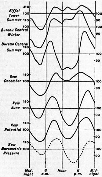
7. In Table III. the diurnal inequality is shown for “winter” and “summer” respectively. In all cases the mean value for the 24 hours is taken as 100. By “summer” is meant April to September at Sodankylä, Greenwich and Batavia; May to August at Kew, Bureau Central (Paris), Eiffel Tower and Perpignan; and May to July at Karasjok. “Winter” includes October to March at Sodankylä, Greenwich and Batavia; November to February at Kew and Bureau Central; November to January at Karasjok, and December and January at Perpignan. Mean results from March, April, September and October at Kew are assigned to “Equinox.”

At Batavia the difference between winter and summer is comparatively small. Elsewhere there is a tendency for the double period, usually so prominent in summer, to become less pronounced in winter, the afternoon minimum tending to disappear. Even in summer the double period is not prominent in the arctic climate of Karasjok or on the top of the Eiffel Tower. The diurnal variation in summer at the latter station is shown graphically in the top curve of fig. 1. It presents a remarkable resemblance to the adjacent curve, which gives the diurnal variation at mid-winter at the Bureau Central. The resemblance between these curves is much closer than that between the Bureau Central’s own winter and summer curves. All three Paris curves show three peaks, the first and third representing the ordinary forenoon and afternoon maxima. In summer at the Bureau Central the intermediate peak nearly disappears in the profound afternoon depression, but it is still recognizable. This three-peaked curve is not wholly peculiar to Paris, being seen, for instance, at Lisbon in summer. The December and June curves for Kew are good examples of the ordinary nature of the difference between midwinter and midsummer. The afternoon minimum at Kew gradually deepens as midsummer approaches. Simultaneously the forenoon maximum occurs earlier and the afternoon maximum later in the day. The two last curves in the diagram contrast the diurnal variation at Kew in potential gradient and in barometric pressure for the year as a whole. The somewhat remarkable resemblance between the diurnal variation for the two elements, first remarked on by J.D. Everett (19), is of interest in connexion with recent theoretical conclusions by J.P. Elster and H.F.K. Geitel and by H. Ebert.

In the potential curves of the diagram the ordinates represent the hourly values expressed—as in Tables II. and III.—as percentages of the mean value for the day. If this be overlooked, a wrong impression may be derived as to the absolute amplitudes of the changes. The Kew curves, for instance, might suggest that the range (maximum less minimum hourly value) was larger in June than in December. In reality the December range was 82, the June only 57 volts; but the mean value of the potential was 243 in December as against 111 in June. So again, in the case of the Paris curves, the absolute value of the diurnal range in summer was much greater for the Eiffel Tower than for the Bureau Central, but the mean voltage was 2150 at the former station and only 134 at the latter.

8. Fourier Coefficients.—Diurnal inequalities such as those of Tables II. and III. and intended to eliminate irregular changes, but they also to some extent eliminate regular changes if the hours of maxima and minima or the character of the diurnal variation alter throughout the year. The alteration that takes place in the regular diurnal inequality throughout the year is best seen by analysing it into a Fourier series of the type

c1 sin(t + a1) + c2 sin(2t + a2) + c3 sin(3t + a3) + c4 sin(4t + a4) + ...

where t denotes time counted from (local) midnight, c1, c2, c3, C4, ... are the amplitudes of the component harmonic waves of periods 24, 12, 8 and 6 hours; a1, a2, a3, a4, are the corresponding phase angles. One hour of time t is counted as 15°, and a delay of one hour in the time of maximum answers to a diminution of 15° in a1, of 30° in a2, and so on. If a1, say, varies much throughput the year, or if the ratios of c2, c3, c4, ... to c1, vary much, then a diurnal inequality derived from a whole year, or from a season composed of several months, represents a mean curve arising from the superposition of a number of curves, which differ in shape and in the positions of their maxima and minima. The result, if considered alone, inevitably leads to an underestimate of the average amplitude of the regular diurnal variation.

It is also desirable to have an idea of the size of the irregular changes which vary from one day to the next. On stormy days, as already mentioned, the irregular changes hardly admit of satisfactory treatment. Even on the quietest days irregular changes are always numerous and often large.

Table IV. aims at giving a summary of the several phenomena for a single station, Kew, on electrically quiet days. The first line gives the mean value of the potential gradient, the second the mean excess of the largest over the smallest hourly value on individual days. The hourly values are derived from smoothed curves, the object being to get the mean ordinate for a 60-minute period. If the actual crests of the excursions had been measured the figures in the second line would have been even larger. The third line gives the range of the regular diurnal inequality, the next four lines the amplitudes of the first four Fourier waves into which the regular diurnal inequality has been analysed. These mean values, ranges and amplitudes are all measured in volts per metre (in the open). The last four lines of Table IV. give the phase angles of the first four Fourier waves.

Table IV.—Absolute Potential Data at Kew (12).

Jan. Feb. March. April. May. June. July. Aug. Sept. Oct. Nov. Dec.

Mean Potential Gradient 201 224 180 138 123 111 98 114 121 153 200 243

Mean of individual daily ranges 203 218 210 164 143 143 117 129 141 196 186 213

Range in Diurnal inequality 73 94 83 74 71 57 55 60 54 63 52 82

Amplitudes of Fourier waves c1 22 22 17 13 18 9 6 6 9 7 14 30

c2 21 33 34 31 22 23 24 26 23 30 17 21

c3 7 10 5 5 3 1 3 2 3 6 5 7

c4 2 3 5 6 4 1 4 3 4 3 2 3

° ° ° ° ° ° ° ° ° ° ° °

Phase angles of Fourier waves a1 206 204 123 72 86 79 48 142 154 192 202 208

a1 170 171 186 193 188 183 185 182 199 206 212 175

a3 11 9 36 96 100 125 124 107 16 18 38 36

a1 235 225 307 314 314 277 293 313 330 288 238 249

It will be noticed that the difference between the greatest and least hourly values is, in all but three winter months, actually larger than the mean value of the potential gradient for the day; it bears to the range of the regular diurnal inequality a ratio varying from 2.0 in May to 3.6 in November.

At midwinter the 24-hour term is the largest, but near midsummer it is small compared to the 12-hour term. The 24-hour term is very variable both as regards its amplitude and its phase angle (and so its hour of maximum). The 12-hour term is much less variable, especially as regards its phase angle; its amplitude shows distinct maxima near the equinoxes. That the 8-hour and 6-hour waves, though small near midsummer, represent more than mere accidental irregularities, seems a safe inference from the regularity apparent in the annual variation of their phase angles.

Table V.—Fourier Series Amplitudes and Phase Angles.

Place. Period. Winter. Summer.

c1. c2. a1. a2. c1. c2. a1. a2.

° ° ° °

Kew 1862-64 0.283 0.160 184 193 0.127 0.229 111 179

” 1898-1904 .102 .103 206 180 .079 .213 87 186

Bureau Central 1894-98 .220 .104 223 206 .130 .200 95 197

Eiffel Tower 1896-98 .. .. .. .. .133 .085 216 171

Sonnblick (22) 1902-03 .. .. .. .. .208 .120 178 145

Karasjok 1903-04 .356 .144 189 155 .165 .093 141 144

Kremsmünster (23) 1902 .280 .117 224 194 .166 .153 241 209

Potsdam 1904 .269 .101 194 185 .096 .152 343 185

9. Table V. gives some data for the 24-hour and 12-hour Fourier coefficients, which will serve to illustrate the diversity between different stations. In this table, unlike Table IV., amplitudes are all expressed as decimals of the mean value of the potential gradient for the corresponding season. “Winter” means generally the four midwinter, and “summer” the four midsummer, months; but at Karasjok three, and at Kremsmünster six, months are included in each season. The results for the Sonnblick are derived from a comparatively small number of days in August and September. At Potsdam the data represent the arithmetic means derived from the Fourier analysis for the individual months comprising the season. The 1862-1864 data from Kew—due to J.D. Everett (19)—are based on “all” days; the others, except Karasjok to some extent, represent electrically quiet days. The cause of the large difference between the two sets of data for c1 at Kew is uncertain. The potential gradient is in all cases lower in summer than winter, and thus the reduction in c1 in summer would appear even larger than in Table V. if the results were expressed in absolute measure. At Karasjok and Kremsmünster the seasonal variation in a1 seems comparatively small, but at Potsdam and the Bureau Central it is as large as at Kew. Also, whilst the winter values of a1 are fairly similar at the several stations the summer values are widely different. Except at Karasjok, where the diurnal changes seem somewhat irregular, the relative amplitude of the 12-hour term is considerably greater in summer than in winter. The values of a2 at the various stations differ comparatively little, and show but little seasonal change. Thus the 12-hour term has a much greater uniformity than the 24-hour term. This possesses significance in connexion with the view, supported by A.B. Chauveau (21), F. Exner (24) and others, that the 12-hour term is largely if not entirely a local phenomenon, due to the action of the lower atmospheric strata, and tending to disappear even in summer at high altitudes. Exner attributes the double daily maximum, which is largely a consequence of the 12-hour wave, to a thin layer near the ground, which in the early afternoon absorbs the solar radiation of shortest wave length. This layer he believes specially characteristic of arid dusty regions, while comparatively non-existent in moist climates or where foliage is luxuriant. In support of his theory Exner states that he has found but little trace of the double maximum and minimum in Ceylon and elsewhere. C. Nordmann (25) describes some similar results which he obtained in Algeria during August and September 1905. His station, Philippeville, is close to the shores of the Mediterranean, and sea breezes persisted during the day. The diurnal variation showed only a single maximum and minimum, between 5 and 6 P.M. and 4 and 5 A.M. respectively. So again, a few days’ observations on the top of Mont Blanc (4810 metres) by le Cadet (26) in August and September 1902, showed only a single period, with maximum between 3 and 4 P.M., and minimum about 3 A.M. Chauveau points to the reduction in the 12-hour term as compared to the 24-hour term on the Eiffel Tower, and infers the practical disappearance of the former at no great height. The close approach in the values for c1 in Table V. from the Bureau Central and the Eiffel Tower, and the reduction of c2 at the latter station, are unquestionably significant facts; but the summer value for c2 at Karasjok—a low level station—is nearly as small as that at the Eiffel Tower, and notably smaller than that at the Sonnblick (3100 metres). Again, Kew is surrounded by a large park, not devoid of trees, and hardly the place where Exner’s theory would suggest a large value for c2, and yet the summer value of c2 at Kew is the largest in Table V.

10. Observations on mountain tops generally show high potentials near the ground. This only means that the equipotential surfaces are crowded together, just as they are near the ridge of a house. To ascertain how the increase in the voltage varies as the height in the free atmosphere increases, it is necessary to employ kites or balloons. At small heights Exner (27) has employed captive balloons, provided with a burning fuse, and carrying a wire connected with an electroscope on the ground. He found the gradient nearly uniform for heights up to 30 to 40 metres above the ground. At great heights free balloons seem necessary. The balloon carries two collectors a given vertical distance apart. The potential difference between the two is recorded, and the potential gradient is thus found. Some of the earliest balloon observations made the gradient increase with the height, but such a result is now regarded as abnormal. A balloon may leave the earth with a charge, or become charged through discharge of ballast. These possibilities may not have been sufficiently realized at first. Among the most important balloon observations are those by le Cadet (1) F. Linke (28) and H. Gerdien (29). The following are samples from a number of days’ results, given in le Cadet’s book. h is the height in metres, P the gradient in volts per metre.

Aug. 9, 1893 { h 824 830 1060 1255 1290 1745 1940 2080 2310 2520

P 37 43 43 41 42 34 25 21 18 16

Sep. 11, 1897 { h 1140 1378 1630 1914 237 2786 3136 3364 3912 4085

P 43 38 33 25 22 21 19 19 14 13

The ground value on the last occasion was 150. From observations during twelve balloon ascents, Linke concludes that below the 1500-metre level there are numerous sources of disturbance, the gradient at any given height varying much from day to day and hour to hour; but at greater heights there is much more uniformity. At heights from 1500 to 6000 metres his observations agreed well with the formula

dV/dh = 34 − 0.006 h,

V denoting the potential, h the height in metres. The formula makes the gradient diminish from 25 volts per metre at 1500 metres height to 10 volts per metre at 4000 metres. Linke’s mean value for dV/dh at the ground was 125. Accepting Linke’s formula, the potential at 4000 metres is 43,750 volts higher than at 1500 metres. If the mean of the gradients observed at the ground and at 1500 metres be taken as an approximation to the mean value of the gradient throughout the lowest 1500 metres of the atmosphere, we find for the potential at 1500 metres level 112,500 volts. Thus at 4000 metres the potential seems of the order of 150,000 volts. Bearing this in mind, one can readily imagine how close together the equipotential surfaces must lie near the summit of a high sharp mountain peak.

11. At most stations a negative potential gradient is exceptional, unless during rain or thunder. During rain the potential is usually but not always negative, and frequent alternations of sign are not uncommon. In some localities, however, negative potential gradient is by no means uncommon, at least at some seasons, in the absence of rain. At Madras, Michie Smith (30) often observed negative potential during bright August and September days. The phenomenon was quite common between 9.30 A.M. and noon during westerly winds, which at Madras are usually very dry and dusty. At Sodankylä, in 1882-1883, K.S. Lemström and F.C. Biese (31) found that out of 255 observed occurrences of negative potential, 106 took place in the absence of rain or snow. The proportion of occurrences of negative potential under a clear sky was much above its average in autumn. At Sodankylä rain or snowfall was often unaccompanied by change of sign in the potential. At the polar station Godthaab (32) in 1882-1883, negative potential seemed sometimes associated with aurora (see Aurora Polaris).

Lenard, Elster and Geitel, and others have found the potential gradient negative near waterfalls, the influence sometimes extending to a considerable distance. Lenard (33) found that when pure water falls upon water the neighbouring air takes a negative charge. Kelvin, Maclean and Gait (34) found the effect greatest in the air near the level of impact. A sensible effect remained, however, after the influence of splashing was eliminated. Kelvin, Maclean and Galt regard this property of falling water as an objection to the use of a water-dropper indoors, though not of practical importance when it is used out of doors.

12. Elster and Geitel (35) have measured the charge carried by raindrops falling into an insulated vessel. Owing to observational difficulties, the exact measure of success attained is a little difficult to gauge, but it seems fairly certain that raindrops usually carry a charge. Elster and Geitel found the sign of the charge often fluctuate repeatedly during a single rain storm, but it seemed more often than not opposite to that of the simultaneous potential gradient. Gerdien has more recently repeated the experiments, employing an apparatus devised by him for the purpose. It has been found by C.T.R. Wilson (36) that a vessel in which freshly fallen rain or snow has been evaporated to dryness shows radioactive properties lasting for a few hours. The results obtained from equal weights of rain and snow seem of the same order.

13. W. Linss (6) found that an insulated conductor charged either positively or negatively lost its charge in the free atmosphere; the potential V after time t being connected with its initial value V0 by a formula of the type V = V0e−at where a is constant. This was confirmed by Elster and Geitel (7), whose form of dissipation apparatus has been employed in most recent work. The percentage of the charge which is dissipated per minute is usually denoted by a+ or a− according to its sign. The mean of a+ and a− is usually denoted by a± or simply by a, while q is employed for the ratio a−/a+. Some observers when giving mean values take Σ(a−/a+) as the mean value of q, while others take Σ(a−)/Σ(a+). The Elster and Geitel apparatus is furnished with a cover, serving to protect the dissipator from the direct action of rain, wind or sunlight. It is usual to observe with this cover on, but some observers, e.g. A. Gockel, have made long series of observations without it. The loss of charge is due to more than one cause, and it is difficult to attribute an absolutely definite meaning even to results obtained with the cover on. Gockel (37) says that the results he obtained without the cover when divided by 3 are fairly comparable with those obtained under the usual conditions; but the appropriate divisor must vary to some extent with the climatic conditions. Thus results obtained for a+ or a− without the cover are of doubtful value for purposes of comparison with those found elsewhere with it on. In the case of q the uncertainty is much less.

Table VI.—Dissipation. Mean Values.

Place. Period. Season. Observer or Authority. a+ q

Karasjok 1903-4 Year Simpson (10) 3.57 1.15

Wolfenbüttel Year Elster and Geitel (39) 1.33 1.05

Potsdam 1904 Year Lüdeling (40) 1.13 1.33

Kremsmüster 1902 Year Zölss (42) 1.32 1.18

” 1903 Year Zölss (41) 1.35 1.14

Freiburg Year Gockel (43) .. 1.41

Innsbruck 1902 Czermak (44) 1.95 0.94

” 1905 Jan. to June Defant (45) 1.47 1.17

Mattsee (Salzburg) 1905 July to Sept. von Schweidler (46) .. 0.99

Seewalchen 1904 July to Sept. von Schweidler (38) .. 1.18

Trieste 1902-3 Year Mazelle (47) 0.58 1.09

Misdroy 1902 Lüdeling (40) 1.09 1.58

Swinemünde 1904 Aug. and Sept. Lüdeling (40) 1.23 1.37

Heligoland (sands) 1903 Summer Elster and Geitel (40) 1.14 1.71

Heligoland plateau ” ” Elster and Geitel (40) 3.07 1.50

Juist (Island) ” Elster and Geitel (48) 1.56 1.56

Atlantic and German Ocean 1904 August Boltzmann (49) 1.83 2.69

Arosa (1800 m.) 1903 Feb. to April Saake (50) 1.79 1.22

Rothhorn (2300 m.) 1903 September Gockel (43) .. 5.31

Sonnblick (3100 m.) 1903 September Conrad (22) .. 1.75

Mont Blanc (4810 m.) 1902 September le Cadet (43) .. 10.3

Table VI. gives the mean values of a± and q found at various places. The observations were usually confined to a few hours of the day, very commonly between 11 A.M. and 1 P.M., and in absence of information as to the diurnal variation it is impossible to say how much this influences the results. The first eight stations lie inland; that at Seewalchen (38) was, however, adjacent to a large lake. The next five stations are on the coast or on islands. The final four are at high levels. In the cases where the observations were confined to a few months the representative nature of the results is more doubtful.

On mountain summits q tends to be large, i.e. a negative charge is lost much faster than a positive charge. Apparently q has also a tendency to be large near the sea, but this phenomenon is not seen at Trieste. An exactly opposite phenomenon, it may be remarked, is seen near waterfalls, q becoming very small. Only Innsbruck and Mattsee give a mean value of q less than unity. Also, as later observations at Innsbruck give more normal values for q, some doubt may be felt as to the earlier observations there. The result for Mattsee seems less open to doubt, for the observer, von Schweidler, had obtained a normal value for q during the previous year at Seewalchen. Whilst the average q in at least the great majority of stations exceeds unity, individual observations making q less than unity are not rare. Thus in 1902 (51) the percentage of cases in which q fell short of 1 was 30 at Trieste, 33 at Vienna, and 35 at Kremsmünster; at Innsbruck q was less than 1 on 58 days out of 98.

In a long series of observations, individual values of q show usually a wide range. Thus during observations extending over more than a year, q varied from 0.18 to 8.25 at Kremsmünster and from 0.11 to 3.00 at Trieste. The values of a+, a− and a± also show large variations. Thus at Trieste a+ varied from 0.12 to 4.07, and a− from 0.11 to 3.87; at Vienna a+ varied from 0.32 to 7.10, and a− from 0.78 to 5.42; at Kremsmünster a± varied from 0.14 to 5.83.

14. Annual Variation.—When observations are made at irregular hours, or at only one or two fixed hours, it is doubtful how representative they are. Results obtained at noon, for example, probably differ more from the mean value for the 24 hours at one season than at another. Most dissipation results are exposed to considerable uncertainty on these grounds. Also it requires a long series of years to give thoroughly representative results for any element, and few stations possess more than a year or two’s dissipation data. Table VII. gives comparative results for winter (October to March) and summer at a few stations, the value for the season being the arithmetic mean from the individual months composing it. At Karasjok (10), Simpson observed thrice a day; the summer value there is nearly double the winter both for a+ and a−. The Kremsmünster (42) figures show a smaller but still distinct excess in the summer values. At Trieste (47), Mazelle’s data from all days of the year show no decided seasonal change in a+ or a−; but when days on which the wind was high are excluded the summer value is decidedly the higher. At Freiburg (43), q seems decidedly larger in winter than in summer; at Karasjok and Trieste the seasonal effect in q seems small and uncertain.

Table VII.—Dissipation.

Place Winter Summer

a+ a− a± q a+ a− a± q

Karasjok 1903-1904 2.28 2.69 2.49 1.18 4.38 4.94 4.65 1.13

Kremsmüster 1903 1.14 1.30 1.22 1.14 1.38 1.56 1.47 1.12

Freiburg .. .. .. 1.57 .. .. .. 1.26

Trieste 1902-1903 0.56 0.59 0.58 1.07 0.55 0.61 0.58 1.13

Trieste calm days .. .. 0.35 .. .. .. 0.48 ..

15. Diurnal Variation.—P.B. Zölss (41, 42) has published diurnal variation data for Kremsmünster for more than one year, and independently for midsummer (May to August) and midwinter (December to February). His figures show a double daily period in both a+ and a−, the principal maximum occurring about 1 or 2 P.M. The two minima occur, the one from 5 to 7 A.M., the other from 7 to 8 P.M.; they are nearly equal. Taking the figures answering to the whole year, May 1903 to 1904, a+ varied throughout the day from 0.82 to 1.35, and a− from 0.85 to 1.47. At midsummer the extreme hourly values were 0.91 and 1.45 for a+, 0.94 and 1.60 for a−. The corresponding figures at midwinter were 0.65 and 1.19 for a+, 0.61 and 1.43 for a−. Zölss’ data for q show also a double daily period, but the apparent range is small, and the hourly variation is somewhat irregular. At Karasjok, Simpson found a+ and a− both larger between noon and 1 P.M. than between either 8 and 9 A.M. or 6 and 7 P.M. The 6 to 7 P.M. values were in general the smallest, especially in the case of a+; the evening value for q on the average exceeded the values from the two earlier hours by some 7%.

Summer observations on mountains have shown diurnal variations very large and fairly regular, but widely different from those observed at lower levels. On the Rothhorn, Gockel (43) found a+ particularly variable, the mean 7 A.M. value being 4½ times that at 1 P.M. q (taken as Σ(a−/a+) varied from 2.25 at 5 A.M. and 2.52 at 9 P.M. to 7.82 at 3 P.M. and 8.35 at 7 P.M. On the Sonnblick, in early September, V. Conrad (22) found somewhat similar results for q, the principal maximum occurring at 1 P.M., with minima at 9 P.M. and 6 A.M.; the largest hourly value was, however, scarcely double the least. Conrad found a− largest at 4 A.M. and least at 6 P.M., the largest value being double the least; a+ was largest at 5 A.M. and least at 2 P.M., the largest value being fully 2½ times the least. On Mont Blanc, le Cadet (43) found q largest from 1 to 3 P.M., the value at either of these hours being more than double that at 11 A.M. On the Patscherkofel, H. von Ficker and A. Defant (52), observing in December, found q largest from 1 to 2 P.M. and least between 11 A.M. and noon, but the largest value was only 1½ times the least. On mountains much seems to depend on whether there are rising or falling air currents, and results from a single season may not be fairly representative.

16. Dissipation seems largely dependent on meteorological conditions, but the phenomena at different stations vary so much as to suggest that the connexion is largely indirect. At most stations a+ and a− both increase markedly as wind velocity rises. From the observations at Trieste in 1902-1903 E. Mazelle (47) deduced an increase of about 3% in a+ for a rise of 1 km. per hour in wind velocity. The following are some of his figures, the velocity v being in kilometres per hour:—

v 0 to 4. 20 to 24. 40 to 49. 60 to 69.

a 0.33 0.64 1.03 1.38

q 1.13 1.19 1.00 0.96

For velocities from 0 to 24 km. per hour q exceeded unity in 74 cases out of 100; but for velocities over 50 km. per hour q exceeded unity in only 40 cases out of 100. Simpson got similar results at Karasjok; the rise in a+ and a− with increased wind velocity seemed, however, larger in winter than in summer. Simpson observed a fall in q for wind velocities exceeding 2 on Beaufort’s scale. On the top of the Sonnblick, Conrad observed a slight increase of a± as the wind velocity increased up to 20 km. per hour, but for greater velocities up to 80 km. per hour no further decided rise was observed.

At Karasjok, treating summer and winter independently, Simpson (10) found a+ and a− both increase in a nearly linear relation with temperature, from below −20° to +15° C. For example, when the temperature was below −20° mean values were 0.76 for a+ and 0.91 for a−; for temperatures between -10° and -5° the corresponding means were 2.45 and 2.82; while for temperatures between +10° and +15° they were 4.68 and 5.23. Simpson found no certain temperature effect on the value of q. At Trieste, from 470 days when the wind velocity did not exceed 20 km. per hour, Mazelle (47) found somewhat analogous results for temperatures from 0° to 30° C.; a−, however, increased faster than a+, i.e. q increased with temperature. When he considered all days irrespective of wind velocity, Mazelle found the influence of temperature obliterated. On the Sonnblick, Conrad (22) found a± increase appreciably as temperature rose up to 4° or 5° C.; but at higher temperatures a decrease set in.

Observations on the Sonnblick agree with those at low-level stations in showing a diminution of dissipation with increase of relative humidity. The decrease is most marked as saturation approaches. At Trieste, for example, for relative humidities between 90 and 100 the mean a± was less than half that for relative humidities under 40. With certain dry winds, notably Föhn winds in Austria and Switzerland, dissipation becomes very high. Thus at Innsbruck Defant (45) found the mean dissipation on days of Föhn fully thrice that on days without Föhn. The increase was largest for a+, there being a fall of about 15% in q. In general, a+ and a− both tend to be less on cloudy than on bright days. At Kiel (53) and Trieste the average value of q is considerably less for wholly overcast days than for bright days. At several stations enjoying a wide prospect the dissipation has been observed to be specially high on days of great visibility when distant mountains can be recognized. It tends on the contrary to be low on days of fog or rain.

The results obtained as to the relation between dissipation and barometric pressure are conflicting. At Kremsmünster, Zölss (42) found dissipation vary with the absolute height of the barometer, a± having a mean value of 1.36 when pressure was below the normal, as against 1.20 on days when pressure was above the normal. He also found a± on the average about 10% larger when pressure was falling than when it was rising. On the Sonnblick, Conrad (22) found dissipation increase decidedly as the absolute barometric pressure was larger, and he found no difference between days of rising and falling barometer. At Trieste, Mazelle (47) found no certain connexion with absolute barometric pressure. Dissipation was above the average when cyclonic conditions prevailed, but this seemed simply a consequence of the increased wind velocity. At Mattsee, E.R. von Schweidler (46) found no connexion between absolute barometric pressure and dissipation, also days of rising and falling pressure gave the same mean. At Kiel, K. Kaehler (53) found a+ and a− both greater with rising than with falling barometer.

V. Conrad and M. Topolansky (54) have found a marked connexion at Vienna between dissipation and ozone. Regular observations were made of both elements. Days were grouped according to the intensity of colouring of ozone papers, 0 representing no visible effect, and 14 the darkest colour reached. The mean values of a+ and a− answering to 12 and 13 on the ozone scale were both about double the corresponding values answering to 0 and 1 on that scale.

17. A charged body in air loses its charge in more than one way. The air, as is now known, has always present in it ions, some carrying a positive and others a negative charge, and those having the opposite sign to the charged body are attracted and tend to discharge it. The rate of loss of charge is thus largely dependent on the extent to which ions are present in the surrounding air. It depends, however, in addition on the natural mobility of the ions, and also on the opportunities for convection. Of late years many observations have been made of the ionic charges in air. The best-known apparatus for the purpose is that devised by Ebert. A cylinder condenser has its inner surface insulated and charged to a high positive or negative potential. Air is drawn by an aspirator between the surfaces, and the ions having the opposite sign to the inner cylinder are deposited on it. The charge given up to the inner cylinder is known from its loss of potential. The volume of air from which the ions have been extracted being known, a measure is obtained of the total charge on the ions, whether positive or negative. The conditions must, of course, be such as to secure that no ions shall escape, otherwise there is an underestimate. I+ is used to denote the charge on positive ions, I- that on negative ions. The unit to which they are ordinarily referred is 1 electrostatic unit of electricity per cubic metre of air. For the ratio of the mean value of I+ to the mean value of I−, the letter Q is employed by Gockel (55), who has made an unusually complete study of ionic charges at Freiburg. Numerous observations were also made by Simpson (10)—thrice a day—at Karasjok, and von Schweidler has made a good many observations about 3 P.M. at Mattsee (46) in 1905, and Seewalchen (38) in 1904. These will suffice to give a general idea of the mean values met with.

Station. Authority. I+ I− Q

Freiburg Gockel 0.34 0.24 1.41

Karasjok Simpson 0.38 0.33 1.17

Mattsee von Schweidler 0.35 0.29 1.19

Seewalchen von Schweidler 0.45 0.38 1.17

Gockel’s mean values of I+ and Q would be reduced to 0.31 and 1.38 respectively if his values for July—which appear abnormal—were omitted. I+ and I− both show a considerable range of values, even at the same place during the same season of the year. Thus at Seewalchen in the course of a month’s observations at 3 P.M., I+ varied from 0.31 to 0.67, and I− from 0.17 to 0.67.

There seems a fairly well marked annual variation in ionic contents, as the following figures will show. Summer and winter represent each six months and the results are arithmetic means of the monthly values.

Freiburg. Karasjok.

I+ I− Q I+ I− Q

Winter 0.29 0.21 1.49 0.33 0.27 1.22

Summer 0.39 0.28 1.34 0.44 0.39 1.13

If the exceptional July values at Freiburg were omitted, the summer values of I+ and Q would become 0.33 and 1.25 respectively.

18. Diurnal Variation.—At Karasjok Simpson found the mean values of I+ and I− throughout the whole year much the same between noon and 1 P.M. as between 8 and 9 A.M. Observations between 6 and 7 P.M. gave means slightly lower than those from the earlier hours, but the difference was only about 5% in I+ and 10% in I−. The evening values of Q were on the whole the largest. At Freiburg, Gockel found I+ and I− decidedly larger in the early afternoon than in either the morning or the late evening hours. His greatest and least mean hourly values and the hours of their occurrence are as follows:—

Winter. Summer.

I+ I− I+ I−

Max.Min.Max.Min. Max.Min.Max.Min.

0.3330.1930.2420.130 0.4300.2440.3330.192

2 PM7 PM2 PM8 PM4 PM9 to4 PM9 to

10 PM 10 PM

Gockel did not observe between 10 P.M. and 7 A.M.

19. Ionization seems to increase notably as temperature rises. Thus at Karasjok Simpson found for mean values:—

Temp. less than −20° −10° to −5° 10° to 15°

I+ = 0.18, I− = 0.36 I+ = 0.36, I− = 0.30 I+ = 0.45, I− = 0.43

Simpson found no clear influence of temperature on Q. Gockel observed similar effects at Freiburg—though he seems doubtful whether the relationship is direct—but the influence of temperature on I+ seemed reduced when the ground was covered with snow. Gockel found a diminution of ionization with rise of relative humidity. Thus for relative humidities between 40 and 50 mean values were 0.306 for I+ and 0.219 for I−; whilst for relative humidities between 90 and 100 the corresponding means were respectively 0.222 and 0.134. At Karasjok, Simpson found a slight decrease in I− as relative humidity increased, but no certain change in I+. Specially large values of I+ and I− have been observed at high levels in balloon ascents. Thus on the 1st of July 1901, at a height of 2400 metres, H. Gerdien (29) obtained 0.86 for I+ and 1.09 for I−.

20. In 1901 Elster and Geitel found that a radioactive emanation is present in the atmosphere. Their method of measuring the radioactivity is as follows (48): A wire not exceeding 1 mm. in diameter, charged to a negative potential of at least 2000 volts, is supported between insulators in the open, usually at a height of about 2 metres. After two hours’ exposure, it is wrapped round a frame supported in a given position relative to Elster and Geitel’s dissipation apparatus, and the loss of charge is noted. This loss is proportional to the length of the wire. The radioactivity is denoted by A, and A=1 signifies that the potential of the dissipation apparatus fell 1 volt in an hour per metre of wire introduced. The loss of the dissipation body due to the natural ionization of the air is first allowed for. Suppose, for instance, that in the absence of the wire the potential falls from 264 to 255 volts in 15 minutes, whilst when the wire (10 metres long) is introduced it falls from 264 to 201 volts in 10 minutes, then

10A = (254 − 201) × 6 − (264 − 255) × 4 = 342; or A = 34.2.

The values obtained for A seem largely dependent on the station. At Wolfenbüttel, a year’s observations by Elster and Geitel (56) made A vary from 4 to 64, the mean being 20. In the island of Juist, off the Friesland coast, from three weeks’ observations they obtained only 5.2 as the mean. On the other hand, at Altjoch, an Alpine station, from nine days’ observations in July 1903 they obtained a mean of 137, the maximum being 224, and the minimum 92. At Freiburg, from 150 days’ observations near noon in 1903-1904, Gockel (57) obtained a mean of 84, his extreme values being 10 and 420. At Karasjok, observing several times throughout the day for a good many months, Simpson (10) obtained a mean of 93 and a maximum of 432. The same observer from four weeks’ observations at Hammerfest got the considerably lower mean value 58, with a maximum of 252. At this station much lower values were found for A with sea breezes than with land breezes. Observing on the pier at Swinemünde in August and September 1904, Lüdeling (40) obtained a mean value of 34.

Elster and Geitel (58), having found air drawn from the soil highly radioactive, regard ground air as the source of the emanation in the atmosphere, and in this way account for the low values they obtained for A when observing on or near the sea. At Freiburg in winter Gockel (55) found A notably reduced when snow was on the ground, I+ being also reduced. When the ground was covered by snow the mean value of A was only 42, as compared with 81 when there was no snow.

J.C. McLennan (59) observing near the foot of Niagara found A only about one-sixth as large as at Toronto. Similarly at Altjoch, Elster and Geitel (56) found A at the foot of a waterfall only about one-third of its normal value at a distance from the fall.

21. Annual and Diurnal Variations.—At Wolfenbüttel, Elster and Geitel found A vary but little with the season. At Karasjok, on the contrary, Simpson found A much larger at midwinter—notwithstanding the presence of snow—than at midsummer. His mean value for November and December was 129, while his mean for May and June was only 47. He also found a marked diurnal variation, A being considerably greater between 3 and 5 A.M. or 8.30 to 10.30 P.M. than between 10 A.M. and noon, or between 3 and 5 P.M.

At all seasons of the year Simpson found A rise notably with increase of relative humidity. Also, whilst the mere absolute height of the barometer seemed of little, if any, importance, he obtained larger values of A with a falling than with a rising barometer. This last result of course is favourable to Elster and Geitel’s views as to the source of the emanation.

22. For a wire exposed under the conditions observed by Elster and Geitel the emanation seems to be almost entirely derived from radium. Some part, however, seems to be derived from thorium, and H.A. Bumstead (60) finds that with longer exposure of the wire the relative importance of the thorium emanation increases. With three hours’ exposure he found the thorium emanation only from 3 to 5% of the whole, but with 12 hours’ exposure the percentage of thorium emanation rose to about 15. These figures refer to the state of the wire immediately after the exposure; the rate of decay is much more rapid for the radium than for the thorium emanation.