Part 1 — CHAPTER VII SYSTEMS OF CO-ORDINATES AND DISTANCE

WE HAVE mentioned in a general way the significance of congruence and of spatial distance. It now remains for us to find a means of defining these concepts in a rigorous mathematical form. We remember that the equality or congruence of two spatial distances between two point pairs and was an indeterminate concept, depending essentially on the behaviour of our measuring rods. An alternative presentation of non-Euclideanism (in the case of two-dimensional geometry) was then found to be afforded by assuming that the distance between points could in all cases be determined by measurements with rigid Euclidean rods; but that, whereas in the case of Euclidean geometry all the points should be considered as existing in the same plane, in the case of non-Euclidean geometry it would be as though the points were situated on a suitably curved surface. Thus, in the case of the earth, the non-Euclidean distance between two points, say New York and Paris, would be given by the Euclidean length of a great circle extending between these points, hence by a curved line following the contour of the earth’s surface. On the other hand, the Euclidean distance between these two same points would be given by the Euclidean length of the straight line joining them and passing, of course, through the earth’s interior.

We now propose to investigate the mathematical expression of distance in two dimensions; we will assume that we are discussing it from the standpoint of Euclidean measurements conducted on surfaces. Let us first consider the case where the surface is an unlimited plane. If we wish to define the position of a point of the plane, we must refer it to some system of reference. Three centuries ago Descartes devised a method whereby this result could be accomplished. He considered two families of Euclidean straight lines which we may call horizontals and verticals, respectively. The lines of these two intersecting families are equally spaced (Euclideanly speaking), so that they form a mesh-system or network of equal Euclidean squares. The scientific name for a mesh-system is co-ordinate system, but the appellation “mesh-system” introduced by Eddington has the advantage of giving a more graphic picture of what is involved. The type of mesh-system constituted by horizontals and verticals introduced by Descartes is called a Cartesian co-ordinate system.

If to each vertical and to each horizontal of the mesh-system we assign consecutive whole numbers from zero on indefinitely, we see that the point of the plane which happens to coincide with the intersection of some particular horizontal and some particular vertical is defined by the numbers which represent the two lines, respectively. In this way every point of intersection is defined by two numbers, and these numbers are called the Cartesian co-ordinates of the point. Of course, by this method we are unable to define the positions of points which do not happen to coincide with the corners of our squares. But there is nothing to prevent us from assuming that between the verticals and horizontals we have mentioned there lie an indefinite number of other similar lines, to which intermediary fractional numbers will be assigned. Henceforth every point of the plane can be regarded as defined by the intersection of some particular horizontal and some particular vertical.

To what extent is it permissible to say that points on the plane have been defined by this method? If we disregard the existence of the co-ordinate system, nothing has been defined, but if we consider the co-ordinate system as given, then every point of the plane can be considered as defined unambiguously. In short, the points are defined not in the abstract, but in relation to the co-ordinate system. There is nothing mysterious about this method of defining the positions of points. Thus, in everyday life, when we agree to meet a friend at the corner of Fifth Avenue and Forty-second Street, we are inadvertently locating our point of meeting in terms of the Cartesian co-ordinate system defined by the avenues and streets. In the present case the co-ordinate system is not strictly Cartesian, since the streets and avenues may not enclose perfectly equal Euclideanly square blocks, but the general principle involved is the same. Needless to say, the definition of our point of meeting would convey no significance were the avenues and streets non-existent. Hence once again we see that it is only relative to the co-ordinate system that points can be defined.

Now, the essential characteristic of the Cartesian procedure is its use of a system of reference represented by separate families of intersecting lines. The fact that the lines we have considered are mutually perpendicular straight lines forming a network of Euclidean squares is of no particular importance. It would be just as feasible, in place of our horizontals and verticals, to select two families of intersecting curves, which we might call the and curves. Of course, our mesh system would now be curvilinear and the spaces enclosed by the meshes would no longer be Euclidean squares, nor even necessarily equal in area. This generalization of Descartes’ method was introduced by Gauss, and for this reason curvilinear mesh-systems are also called Gaussian mesh-systems. As before, every point will be defined by the numbers designating the two curves of either family, that is, by the numbers designating the curve and the curve which intersect at this point; and these two numbers will be called the Gaussian numbers or co-ordinates of the point.

The necessity of generalising Cartesian co-ordinates by introducing Gaussian ones arises from the fact that Cartesian mesh-systems of equal squares can be traced only on a plane and could never be drawn on a curved surface, like that of a sphere, for example. Hence, were we to ignore the use of Gaussian mesh-systems, it would be impossible for us to localise points on a curved surface, by means of a mesh-system applied on the surface. The nearest approach to a network of squares on the surface of a sphere would be a network of meridians and parallels, and such a network is not one of equal Euclidean squares; it is a curvilinear or Gaussian mesh-system tapering to points at the North and South Poles.

As a matter of fact, we also make use of Gaussian co-ordinates in everyday life. Such is the case when we state that the position of a ship is so many degrees of latitude and so many degrees of longitude; our mesh-system, being one of meridians and parallels, is a Gaussian one, and the latitude and longitude of the ship constitute its Gaussian co-ordinates.

Having determined how the positions of points may be defined on any surface in terms of some mesh-system, let us now see how it is proposed to express the distance between two points, as measured over the surface with rigid Euclidean rods. Here we must proceed with the utmost caution. Let us recall exactly what is involved. Any definite line is one along which remains constant while varies continuously, and inversely any definite line is one along which remains constant while varies continuously. In much the same way, on the earth’s surface a latitude line or parallel is one along which the latitude remains constant and the longitude varies, whereas a longitude line or meridian is one along which the reverse is true.

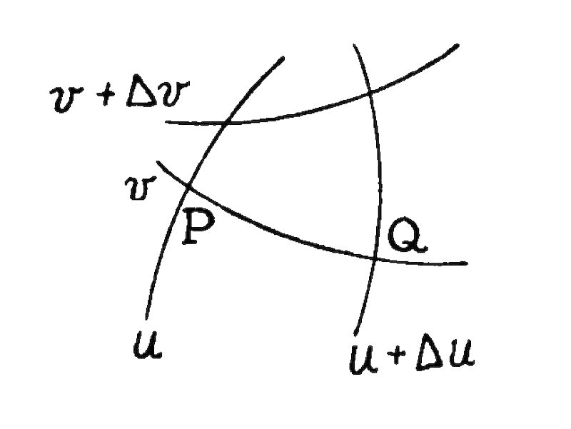
Fig. II

Suppose, then, we wish to express the distance between two points and , defined by the intersections of a certain line with two successive lines (Fig. II). The co-ordinates of the two points are () and (), respectively, where represents the increase in the value of as we pass from to on the line.

On no account may we say that the distance (which we shall call ) is given by the value , for is nothing but a difference between numbers serving to localise points; it has nothing in common with a distance. In order to dispel any doubts on this score, we may notice that if we compare the lines to parallels and the lines to meridians, the points and will be given by the intersections of two consecutive meridians with the same parallel. In this case would correspond to the difference in longitude between the two points; and obviously a difference in longitude is no criterion of a distance, since for the same difference in longitude the distance decreases from equator to pole. In short, the distance between and cannot be fully determined by .

Yet, on the other hand, just as the distance between two points lying on the same parallel is affected by their difference in longitude, so now the distance between and must be a function of the co-ordinate difference . A sufficiently general expression of a quantity when defined in terms of another quantity on which it depends is given by where , , are appropriate magnitudes. If, however, we consider points exceedingly close together, becomes exceedingly small in value, and as a result and , etc., are many times smaller still. At the limit, therefore, when the two points are at an infinitesimal distance apart, the higher powers of become so insignificant that they can be neglected in comparison with . We thus obtain , and in order to specify that we are considering infinitesimal distances we replace the symbol by and obtain It is customary to designate by so that, using squares, our formula becomes

And now we have to consider an important question. What is ? What does it represent? We do not propose to enter into its full mathematical significance, but we may mention certain of its important characteristics. In our illustration of meridians and parallels, let us consider the various points of intersection defined by the intersections of the successive parallels with two fixed meridians. The difference in longitude between these various point pairs will, of course, be constant and will be given by the same invariable quantity . Inasmuch as the distance between these point pairs varies from pole to equator, we see from that must vary in an appropriate way as we consider various portions of the sphere’s surface. In fact, owing to the constancy of , we must have proportional to . If, then, the meridians were parallel lines instead of tapering together towards the poles, would remain constant. Whence it follows that a knowledge of the way varies from point to point yields us information on the shape of the mesh-system, and inversely the lay of the mesh-system yields us information as to the value of from place to place.

Then again, if, leaving our two points and fixed, we select some new mesh-system, may change in value, and in fact a difference may also appear, since with a change of mesh-system there is no reason why and should still lie on the same curve. Hence we must conclude that even at a fixed point of our surface the value of will be subject to change when we vary our mesh-system.

Precisely the same arguments would apply were we to consider the expression of the distance between two infinitely close points on the same curve. We should then obtain , where is a magnitude generally differing from .

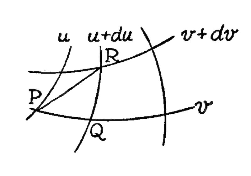
Fig. III

We must now consider the more general case where our two points lie on different and curves (Fig. III). From what precedes we know that the squared distance is given by and that the squared distance is expressed by . But this information is obviously insufficient to tell us what the squared distance will be, since this distance will also be affected by the slant of the lines and . Some new magnitude will obviously have to be introduced in order to specify the value of this slant; and the new magnitude considered will be called and . Under the circumstances, the squared distance of the infinitesimally near points and can be written but as and are found to be always identical we have We may write this formula more concisely by referring to as and to as . In this case our formula becomes where indicates summation and where for and we substitute the values 1 and 2 in all possible ways. This most important mathematical expression was discovered by Gauss; it is destined to play a part of paramount significance in the physical theory of relativity.

In order to understand the geometrical meaning of , let us consider the special case of a diamond-shaped mesh-system, where the co-ordinate lines make an angle (Fig. IV). Elementary geometry teaches us that

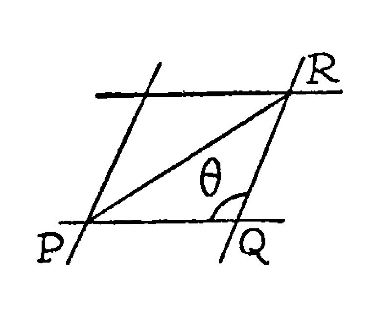
Fig. IV

The lines being always equally spaced, and remain constant throughout the mesh-system; hence we may put them equal to unity and write In this formula we have from which we see that represents the cosine of the angle formed by the and lines, at the point where is calculated.[26] Inasmuch as , we see that where the and lines are perpendicular, vanishes. Hence, whenever we have an expression of , such as from which is absent, we may be certain that the and lines are orthogonal at the point for which has been calculated.

If the and lines remain perpendicular throughout the entire mesh-system, will vanish not only for one particular point, but for all points of the surface.

Let us now consider the particular case of a Cartesian mesh-system of equal squares. In this case, the and lines being orthogonal and equally spaced, we have and constant, with vanishing. Hence we may replace and by unity, and we obtain a result in complete agreement with the Pythagorean theorem of the square of the hypothenuse.

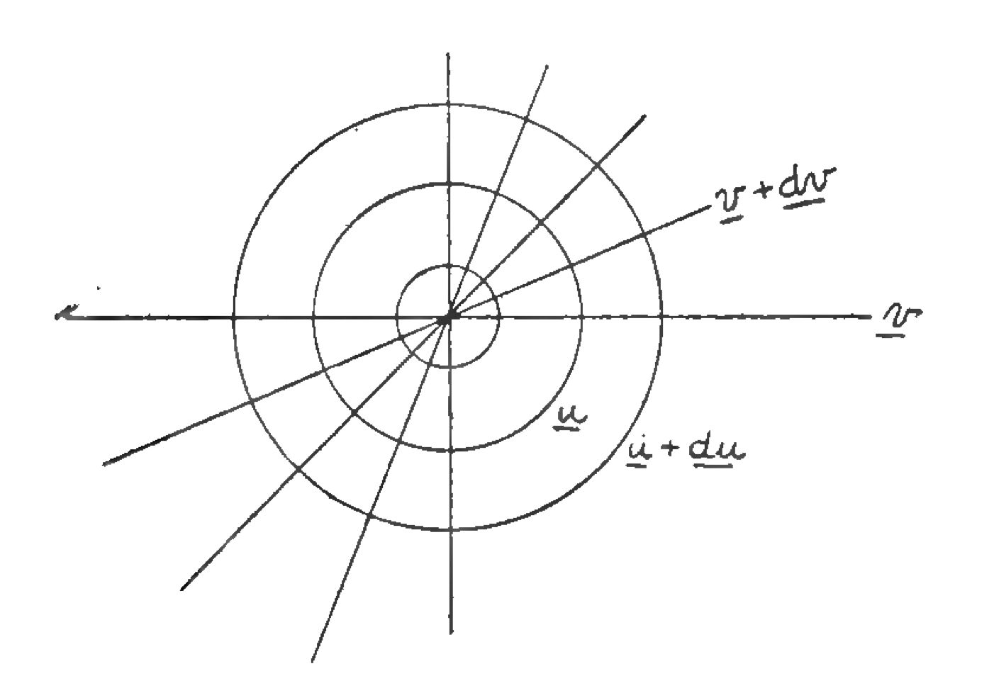
Fig. V

Suppose, now, that on this same plane we were to trace another type of co-ordinate system, one known as a polar system (Fig. V). It is constituted by symmetrically disposed v lines radiating from a central point . The lines are then given by equally distanced concentric circles having as centre. Under the circumstances the expression for becomes In other words, we have proving once again that the values of the ’s vary with our choice of a co-ordinate system. As before, vanishes for the same reasons as previously stated, namely, because the lines of our mesh-system are orthogonal at their intersections.

Finally, we may consider the mesh-system defined by the parallels and meridians on a sphere, where we may assume that gives a parallel and gives a meridian. Here we have so that

From these various examples the following conclusions may be drawn:

1°. When a definite mesh-system has been traced on a surface and its lines numbered consecutively, every point of the surface is defined unambiguously by its two numbers (its two Gaussian numbers or co-ordinates). These numbers represent, of course, those of the respective and curves at whose intersection the point stands. A variation in the shape or in the numbering of the and lines entails a change in the co-ordinate numbers of any given point on the surface.

2°. Alongside of these two Gaussian numbers at every point defining the positions of points in the mesh-system, there exist four numbers, at every point, namely , , , . But as and are always identical, we have only three of these magnitudes to consider. The values of these ’s at a point vary when we change our mesh-system. In the majority of cases they also vary from place to place throughout the same mesh-system. If, however, the meshes are always orthogonal at their points of intersection, vanishes at every point of the surface. If the and lines always have the same slant over the surface and are always equally spaced, the three ’s will remain constant throughout; their values being given by 1, , 1. If the mesh-system is Cartesian, hence forms equal squares , of course, vanishes while, as before, and remain constantly equal to unity.

3°. The value of the square of the distance between two infinitesimally distant points is given by where the values of the ’s and of and will vary when the mesh-system is changed or when we consider different regions of the same mesh-system. The only case in which the ’s will remain constant is when the mesh-system is of the uniform type, that is, a network of two families of parallel lines intersecting one another.

It is a remarkable fact that although everything entering into the expression of varies when we change our mesh-system, yet the value of as defining the value of the square of the distance between two infinitesimally distant points remains unchanged. In other words, is a scalar, an invariant. This allows us to place a new interpretation on the numbers; they appear to act as correctives counterbalancing the variations of and . If we compare the variations in the values of and when the mesh-system is changed, to the advance of a squirrel in a drum, we see that the action of the ’s is similar to a backward revolution of the drum, offsetting the squirrel’s advance, so that the squirrel remains motionless in space.[27]

Now, up to this point we have been considering the expression of a distance between infinitely close points, but in practice we also wish to establish the length of an extended curve traced on the surface. In this case we proceed from point to point along the curve, computing the successive infinitesimal distances , then summating them, or, as it would be more proper to say, integrating them. We thus obtain . Also we may state that the area of an infinitesimal parallelogram formed by two-line elements and is given by Here again we may calculate any finite area by a process of integration, so we see that the finite geometry of the surface can be studied by concentrating our attention on infinitesimal portions and then extending our results from place to place. In short, the method reduces to an application of the differential calculus to geometrical problems, and for that reason is named differential geometry.

Powerful as this method of differential geometry has proved to be, there are cases in which it cannot be applied. However, as in the problems of physics with which we shall be concerned, difficulties do not arise, we need not dwell on a number of special cases which in the present state of our knowledge are of interest only to the mathematician.[28]

And now we come to the main body of Gauss’ discoveries. We have seen that on a given surface the values of the three ’s at any point, or, more correctly, their variations in value from point to point, are defined by our choice of a mesh-system. But we know that a mesh-system, though in large measure arbitrary, is yet not completely independent of the nature of the underlying surface. For instance, a Cartesian mesh-system of equal squares, or again a diamond-shaped one, both of which hold on a plane, cannot be traced on a sphere. Neither can a network of meridians and parallels which holds on a sphere be traced on a plane. For this reason the representation of the disposition of oceans and continents is necessarily distorted in some way or other when given on a flat map.

In short, every species of surface possesses an infinite aggregate of possible mesh-systems, but those systems which are applicable to one type of surface are never applicable to surfaces of any other type. Inasmuch as the Cartesian mesh-system and the diamond-shaped variety are the only ones that entail the constancy of the three ’s throughout the surface, and inasmuch as such co-ordinate systems can be traced only on a plane or on surfaces derived therefrom without stretching (cylinder, cone), we see that the constancy of the three ’s is characteristic of Euclideanism. This does not mean, of course, that all co-ordinate systems traced on a plane yield constant values for the three ’s; it simply means that on a plane it is always possible to trace a Cartesian mesh-system, whereas on all other types of surfaces the task is impossible.

All this goes to prove that the curvature of a surface must exert a modifying influence on the -distribution, since when the surface is curved no constant distribution is possible. We must infer, therefore, that the -distribution is governed by two separate influences; first, by the lay of the mesh-system over the surface; secondly, by the intrinsic curvature of the surface from place to place. Gauss realised the importance of separating these two influences and of determining in what measure respectively they affected the -distribution.

Obviously, if it were possible to discover some mathematical expression connecting the ’s at one point with the ’s at neighbouring points, and if this mathematical expression remained invariant in value to a change of mesh-system in spite of the variations of the individual ’s which must accompany the change of mesh-system, we should be in the presence of a magnitude which, transcending our choice of a mesh-system, would refer solely to the shape of the surface itself, i.e., to its curvature at the point considered. But before we investigate the nature of Gauss’ discoveries, certain elementary notions must be recalled.

We know that the curvature of a circle at every point of its circumference is a constant given by , where is the radius of the circle. But if in place of a circle we trace any arbitrary curve on our plane, the curvature will vary from point to point along the curve. The curvature of the curve at given point is then defined by the a certain circle which is tangent to the curve at the point . As a matter of fact there exist an indefinite number of circles of varying radii lying tangent to the curve at ; but among these circles one stands out prominently in that it is, so to speak, more perfectly tangent than all the others. Whereas the tangent circles intersect the curve in two points coinciding at , this privileged circle intersects it in three such points. It is called the osculating circle (osculare meaning to kiss in Latin). The curvature of the curve at is defined by the curvature of its osculating circle at . Calling the radius of this osculating circle, the curvature of the curve at is thus given by (Fig. VI).

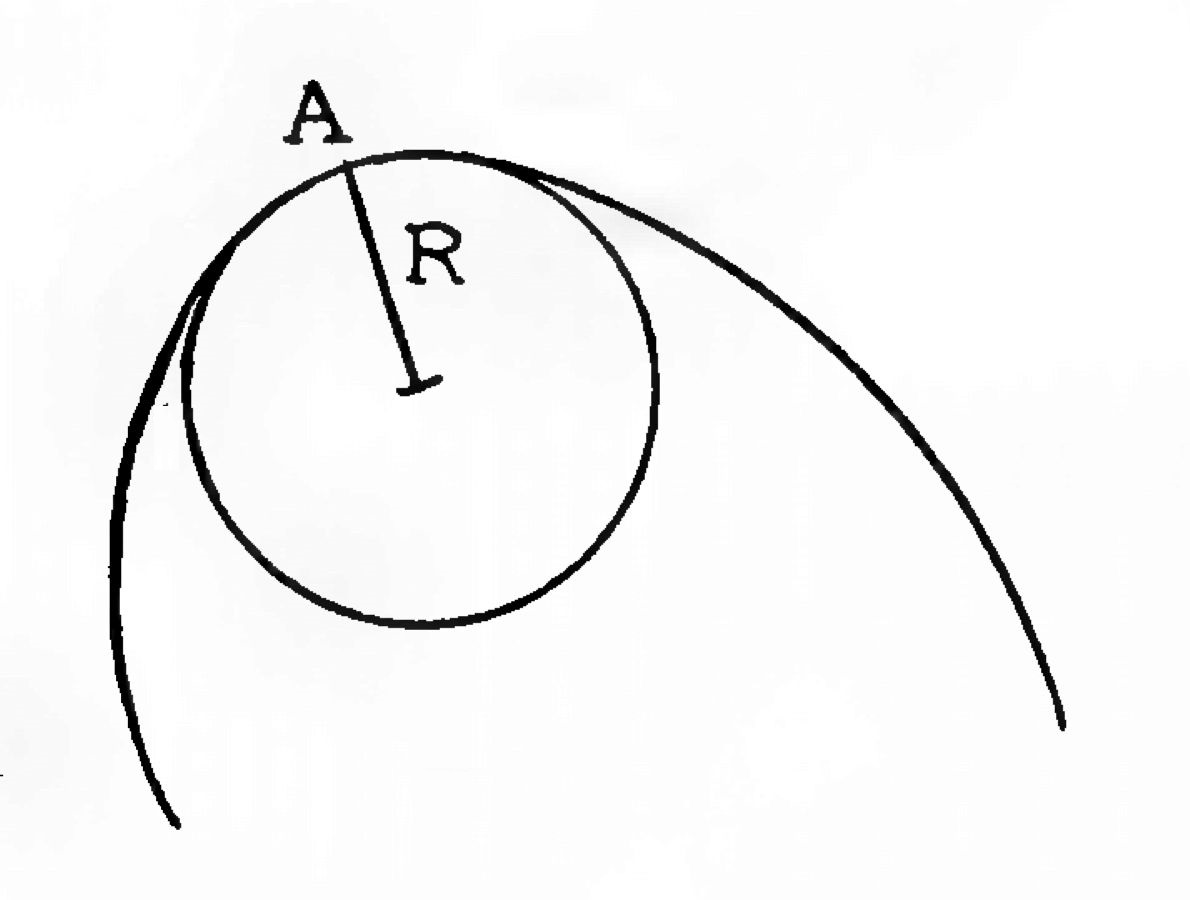
Fig. VI

We must now pass to the curvature of a surface. At a point on the surface where the curvature is to be computed we trace a normal to the surface. Then through this normal we trace a plane, which of course intersects the surface along a plane curve. We assume this normal plane to revolve round the normal as axis and we thus obtain a series of plane curves of intersection defined by the normal plane and surface. Each one of these curves passing through the point possesses a definite curvature at , and this curvature can be computed through the medium of the corresponding osculating circle.

Here a geometrical fact is evidenced. It is found that in the general case there exist two remarkable positions of the intersecting normal plane, perpendicular to one another and therefore sectioning the surface along two curves (1) and (2) orthogonal to each other at . The curvature of one of these curves, say, the curve (1), is less than that of all other curves obtained by revolving the plane round the normal at , while the curvature of the second curve (2) is greater than all others. These two curvatures are called the two principal curvatures of the surface at the point and are designated by and respectively.

We then define the total curvature or the Gaussian curvature of the surface at the point by the product . If our surface is a sphere we have , hence the Gaussian curvature becomes or more simply , where is the radius of our sphere; but in the general case, and are unequal. According to the nature of the surface the two principal curvatures may be of the same or of opposite signs. When of the same sign, the total curvature is obviously positive; hence the surface is said to manifest positive curvature at the point considered. The sphere and ellipsoid are illustrations of surfaces presenting a positive curvature throughout. When, however, the surface is saddle-shaped, the two principal curvatures are of opposite sign; the total Gaussian curvature is then negative, and we have a surface of negative curvature at the point considered.

And now let us return to Gauss’ discoveries. We saw that the distribution of the ’s over the surface was affected both by our choice of a mesh-system traced on the surface and by the intrinsic nature or curvature of the surface from point to point. Then we also mentioned that if it were possible to discover some mathematical expression connecting the ’s at a point with the ’s at neighbouring points, and that if this mathematical expression remained invariant in value to a change of mesh-system in spite of the variations of the individual ’s which accompany the change of mesh-system, we should be in the presence of a magnitude which, transcending our choice of mesh-system, would refer solely to the shape of the surface itself, i.e., to its curvature at the point considered. This important mathematical invariant, built up with the ’s, was discovered by Gauss; it is generally designated by the letter and is referred to as the scalar or invariant of curvature at the point . Gauss then proved that this scalar of curvature was none other than minus twice the total curvature defined previously. Hence we may write: Aside from a constant factor, these two curvatures are thus the same, so that we shall often refer to as the Gaussian curvature, even though the appellation is not strictly accurate.[29]

Before proceeding farther, we must recall that the method we have followed of investigating the geometry of surfaces and using Euclidean rigid rods for the purpose of conducting measurements over the surface, leads to the same geometrical results as would be obtained by an exploration of a two-dimensional space (of a plane, for example) by means of non-Euclidean rods. If, therefore, we conducted measurements with non-Euclidean measurements over a plane, we should of course obtain a non-Euclidean geometry; and the Gaussian curvature of the plane would no longer vanish, as it would were we to make use of the Euclidean measuring rods.[30]

In terms of our non-Euclidean measurements the same plane would be curved. We see, therefore, that the non-vanishing of the Gaussian curvature does not necessarily represent curvature in the usual visualising sense. It represents more truly a relationship between the surface and the behaviour of our measuring rods; in other words, it represents non-Euclideanism, and the word “curvature” is apt to be misleading. In a general way, therefore, we may state that the type of geometry of our two-dimensional space from place to place is defined by the value of the Gaussian curvature from point to point, hence by the law of -distribution throughout the space; and that when the space is Euclidean, the -distribution is always such that the Gaussian curvature vanishes at all points, regardless of the particular mesh-system selected.

Now all these discoveries of Gauss relating to a two-dimensional space were extended by Riemann to spaces of any number of dimensions. Riemann found that for spaces of more than two dimensions the results became very much more complex. In the case of a space of dimensions we of course require Gaussian co-ordinates to define the position of a point in our mesh-system, which now becomes -dimensional. As before, we can conceive of Cartesian and Gaussian mesh-systems, the former being a generalisation to dimensions of our network of Euclidean squares. As for the invariant mathematical expression of the square of a distance between two points, it now contains a greater number of terms. In the case of three-dimensional space we have no longer three separate quantities at every point; this number is increased to six. In the case of a four-dimensional space it is increased to ten, and in the case of an -dimensional space to .

Owing to the importance of a four-dimensional extension in the theory of relativity, we shall write out the expression of the square of the distance for a four-dimensional space. If we call , , , the four differences between the four Gaussian co-ordinates of our two infinitely close points and and designate the ten numbers at every point by , , etc., we have or, more concisely, where we give to and all whole values from 1 to 4, permuting them in all possible ways. Accordingly, in what follows, we shall refer to the ’s as the ’s.

Proceeding by the same method as we did in the case of two dimensions, we find that there now exist several invariant types of relations between the ’s at every definite point and their variations in value at all points near this one. The values of these expressions remain unchanged when we alter our mesh-system; hence, as in the case of the Gaussian curvature for two-dimensional space, they refer to the geometry of the space itself and not to our choice of mesh-system. One of these invariant expressions is the generalisation of the Gaussian curvature extended to four dimensions. The others refer to new types of curvatures which appear only in spaces of more than two dimensions. It is impossible to represent these curvatures with a two-dimensional surface because they then become identified with the ordinary Gaussian curvature.[31] For this reason it was only when curved spaces of more than two dimensions were studied that these new forms of curvature were brought into prominence.

From what has been said we may anticipate marked complications when we wish to study the geometry of a space of more than two dimensions. Thus, we saw that in a two-dimensional space the Gaussian curvature fully defines the geometry of the space. For instance, if the Gaussian curvature vanishes throughout, the surface is Euclidean or at least flat.[32] In the same way, if the Gaussian curvature is an invariable positive or negative number throughout, the surface is one of constant curvature, either positive, as with a sphere, or negative, as with a pseudosphere.

But when we consider spaces of more than two dimensions, a knowledge of the generalised Gaussian curvature throughout the space is no longer sufficient to fix its geometry. While this curvature may vanish or present the same non-vanishing value throughout, we cannot infer therefrom that the space is necessarily flat or of constant curvature. Thus, whereas the vanishing of the generalised Gaussian curvature is a necessary condition for the space to be flat, it is by no means sufficient. There is still room for a large measure of indeterminateness in the actual geometry of the space.

For the geometry of a space of more than two dimensions to be determined fully, we must state the values of the components of the tensor (mentioned in the note); there being twenty such components at every point for a four-dimensional space. We may note that, contrary to the Gaussian curvature , is not invariant. It splits up into components each one of which may vary in value when the mesh-system is changed. Yet, in spite of this variability, still defines the curvatures of the space, hence still refers to something that is intrinsic and irrelevant to our choice of mesh-system. Such is one of the characteristics of a tensor. This particular tensor of twenty components (in a four-dimensional space) is known as the Riemann-Christoffel tensor.[33] Curiously enough, it was discovered by Riemann, not when investigating the geometry of space, but when considering a problem in heat.

Only when every one of these twenty components of the tensor vanishes at every point is it possible to assert that the four-dimensional space is Euclidean, or at least flat. Thus, whereas for two dimensions Euclideanism was ensured when one condition was satisfied at every point, namely, the vanishing of the Gaussian curvature, , on the other hand, when we step up to four dimensions, twenty conditions are needed, and these are given by the vanishing at every point of the twenty expressions which in their aggregate constitute the Riemann-Christoffel tensor .

We may also mention that in addition to the Riemann-Christoffel tensor , Einstein has made use of the other tensor (previously discovered by Ricci), which in four-dimensional space is defined by ten separate relations between the values of the ’s at a point and their values at neighbouring points. The vanishing of this other tensor at every point, that is to say, the vanishing of the ten new component expressions at every point, is insufficient in itself to ensure the Euclideanism of the space; although, of course, this vanishing imposes certain restrictions on the space’s non-Euclideanism. These restrictions are less severe than those defined by the vanishing of the twenty components of the Riemann-Christoffel tensor, which ensures perfect flatness; on the other hand, they are more stringent than those imposed by a mere vanishing of the Gaussian curvature .[34]

Turning to the physical significance of the numbers, we may note that it is these magnitudes which enter into the expression of a distance, hence which serve to define congruence. If we are dealing with a purely amorphous continuum in which no particular definition of congruence or distance is pressed upon us by nature, there can exist no particular distribution of numbers inherent in the continuum. But if, on the other hand, as in the case of space, or, better still, of Einstein’s four-dimensional space-time, a precise definition of practical congruence is imposed upon us by nature—if, in other words, our continuum, in place of being amorphous, possesses a definite metrics or structure—there will exist a -distribution inherent in the continuum, and this distribution will define its metrical field.

The same arguments would apply to the structural tensors of curvature of the continuum, namely, to , to and to . If the continuum is amorphous, these structural tensors, together with the ’s that compose them, are meaningless until we have decided upon some theoretical type of congruence of geometry; and even then they represent characteristics of structure that are as conventional as the geometry we have selected. But if, on the other hand, a definite metrics exists in the continuum, then these structural tensors represent curvatures of the continuum, which we may regard as physically existent and no longer as purely conventional.