PART II. MOTION OF COMETS THROUGH THE SYSTEM.

I. It was not till the period, when a general spirit of inquiry burst forth, and men began to seek, from observation, the acquaintance with nature, which mere conjecture had before supplied, that these extravagant prejudices with respect to Comets began to be shaken. But the great barrier to be overcome, was the universal acquiescence in the doctrines of Aristotle; for his name reigned paramount, in every department of learning; and it is a curious fact, that, so late as the seventeenth century, in some of the universities of Europe, the professors were required to declare upon oath their belief, that those doctrines were infallible, and promise, in their public lectures, to follow Aristotle as their only guide. The first circumstance which contributed to change the tide of popular opinion, were two facts ascertained with respect to the direction of the tail, and the distance of Comets from the earth. Appian, between the years 1531 and 1539, had attentively observed several comets; and he was particularly struck with the discovery, that all of them, in every part of their course, constantly kept their tails in a direction opposite to the sun. As the same fact was soon remarked, in many other comets, its general occurrence led astronomers to suspect some relation between them and the sun, on which the formation of the tail, as well as the motion of the comet itself, might probably depend. Another discovery, still more important, was soon afterwards made, which served to confirm this idea. Tycho Brahe, who had the advantage of possessing better instruments for observation, than those hitherto used by astronomers, occupied himself sedulously in examining the Comet of 1577; he found its parallax to be no more than 20′; and hence he was enabled to establish the extraordinary fact, that the comet, so far from occupying the atmosphere of the earth, according to universal belief, must have been nearly three times more distant than the moon, (the moon’s parallax being 54′). In accordance with this discovery, Tycho was led to consider these bodies as formed by exhalations from the planets, moving in the heavens like them, though of a highly attenuated constitution; and he supposed them to revolve round the sun in orbits, beyond Mercury and Venus: In this manner, he attempted to account for the inequalities in the motion of Comets, by supposing their orbits not so uniformly circular, as those of the planets, but resembling more the form of an egg; an opinion which, although originating in mere conjecture, may be deemed nearly a divination of the truth.

Thus, then, by progressive steps, were astronomers able to demonstrate the absurdity of the doctrines which had so long prevailed, and approached to some knowledge of the place really occupied by comets in the system. But little advance could as yet be made beyond this point; for, with respect to the manner in which Comets move through the planetary regions, or still more, as to their formation and origin, the conjectures even of the wisest were extremely crude. The human mind, in the first exercise of its powers, after a long period of inactivity, is ever prone to indulge in the wildest speculations. Kepler himself, the disciple of Tycho Brahe, and the father of modern astronomy, had no idea that comets are guided in their course, by the same simple and universal laws, which he had found to regulate the motions of the planets; but entertained the truly ridiculous belief, that they are monsters moving in the celestial spaces, engendered by a certain animal faculty existing in the air. However, notwithstanding this extravagant conjecture, Kepler was very attentive to the motions of these strange bodies, and found that they were not confined in their course to straight lines, as was imagined. James Bernouilli, an Italian astronomer, started the idea that they might be the satellites of some distant planet, which are always too far removed to be visible from the earth, unless when they come into a certain portion of their course. The theory of Tycho Brahe, however, that comets move like the planets, in orbits nearly circular, seems, perhaps from its simplicity, to have obtained the most general credit; but all astronomers were now agreed upon one point, on account of the small parallax which comets were discovered to possess, that whatever might be the actual line of their course, they must be situated far beyond the atmosphere of the earth.

But, that the path of Comets could not be represented by a circular orbit, was soon shewn by more accurate and extended observations. Hevelius was the first who distinctly proved this fact, by delineating on a planisphere, the apparent motion of several comets. The result showed, that although in one part of its track, the orbit of a comet may be circular, yet that, in general, it more nearly approaches a straight line; and therefore he concluded, that the cometary orbits must be elongated curves, of a lenticular shape. Hevelius being disposed, with Tycho, to consider the comets as planetary meteors moving through the celestial regions, it occurred to him, that their course might be analogous to the path of bodies, projected in our own atmosphere: and as he observed with regard to the latter, that, solicited by two forces, viz. their own original impulse, and the attraction of the earth, they describe a parabola, he thought that the trajectories of comets, must be determined by similar laws. He therefore investigated what are the forces, which may cause a comet to pursue its course: one is the force of impulsion, by which, according to him, they quit the atmospheres of the planets; another is, their natural tendency towards the sun; and in this consideration he found a confirmation of his opinion. He even went so far as to remark, that the velocity of comets is greatest at the point, where the curvature of their orbit is the most considerable, and where the line drawn to them from the sun, is perpendicular to the curve;—in short, at the vertex of the parabola. From this, Hevelius deduced, that the sun itself, must be situated in the plane of the Comet’s orbit, and occupy some point in the line which is termed the axis of the parabola. But though Hevelius was thus able to arrive at the important fact, that comets, in their progress round the sun, describe a conic section in common with the planets, he was able to proceed no farther. The determination of that orbit in the case of any particular comet, was yet reserved for a more advanced period of the science, when astronomers should be both more unanimous in their opinions regarding the paths of comets, and better able, by the possession of instruments, to observe their course.

Cassini, however, entertained very different ideas. He revived Kepler’s notion, that these bodies move in straight lines; and was even able to give a semblance of truth to this absurd opinion, by predicting, with wonderful success, the path which several comets would follow through the heavens. This coincidence of fact with theory, a theory so wide from the truth, is not however, very surprising; seeing that, during a considerable portion of their orbit, the curve does not materially differ from a straight line. But why Comets, after having reached the sun, should return towards the same quarter of the heavens, whence they had come in their approach, was a fact which Cassini in vain sought to reconcile with his theory; and he therefore endeavoured to make out, that when a comet did not seem to fall into the body of the sun as he imagined, but to describe a track round it, this was a different Comet altogether, which had never been observed before. No farther approximation was made to the truth, till the great Comet of 1680 appeared.

This Comet, which, from its magnitude and brilliancy, excited among the vulgar the most feverish anxiety and even terror, proved an object of no less interest and profound attention to astronomers. Its course was carefully watched, and various theories were framed to account for its motions, and ascertain its orbit. The merit of having first started the idea, that the orbit of this comet was a parabola, has been commonly ascribed to Döerfield, an obscure clergyman of Saxony; who, adopting the opinion of Hevelius, only with this difference, that Döerfield supposed the sun to occupy the focus itself of the parabola, published his theory in a small work in the year 1680. If, however, merit is at all due to a discovery, founded rather on vague conjecture than any certain data, that merit must be ascribed to our own countryman, Henry Percy, Earl of Northumberland, who, in the beginning of the same century, advanced much nearer the truth, by assuming an ellipse as the curve of a comet’s orbit, of which the sun is in one of the foci‍‍55.

But the period was now at hand, when, according to the prediction of Seneca, a person should at length appear, to point out the proper path of discovery; and who, like those very comets whose laws he explained when they issue from the dark abysses of space to their perihelion, would at once emerge from this undigested chaos of conjecture, into the full light of truth. It was Newton, who, by the inspirations of his comprehensive genius, was the first to divine the nature of those mysterious bodies; and who, subverting the futile and fanciful notions of preceding ages, established a theory of his own, upon the immutable basis of demonstration. Having already discovered, that gravitation is the great principle by which all the planetary motions are governed, Newton had little doubt that comets, which were now known to be situated far beyond the earth’s atmosphere, would be found to afford the most decisive proof of the universality of this fundamental law. Led to this supposition on the ground of the strongest analogy, an opportunity only was wanting to try it by the test of observations, which astronomical records were yet too imperfect to supply. The Comet of 1680 above mentioned, afforded that opportunity; and from the diligent manner in which it was watched during its progress round the sun, Newton at length had the satisfaction of finding, that it was guided in its track by exactly the same laws as those which regulate the movements of the planets.

II. In fact, this result was a necessary, and it may even be said an obvious consequence of the principle of universal attraction, which, independent of the more cautious but circuitous method of induction, Newton might with certainty have anticipated: since it follows from the theory of central forces, that a body moving round another by the action of a power (such as gravitation) tending to its centre, must describe a conic section, of which the latter body is the focus. With respect to all bodies following a curvilineal track, there are two forces alone to be considered. The first is the centripetal force, which is the immediate effect of that attraction by which it is drawn towards a certain point; and the next is the centrifugal force, arising and inseparable from a curvilineal track. Suppose that the body is first put in motion by some projectile force, whose action would cause it to move uniformly in a straight line; by the operation of the central force, however, it is continually deflected from this rectilineal path, and therefore the body is compelled to circulate in a curvilineal track around the central or attracting point. The orbit which is actually followed must evidently pass through the points where the centripetal and centrifugal forces exactly counterbalance each other; and hence it will just depend on the mutual relation of those opposite forces, whether the curve described shall be a circle, a parabola, a hyperbola, or an ellipse. If, for instance, the intensities of the central and projectile forces are exactly equal, then the curve produced by their combined operation will be a circle: If, however, we suppose the projectile force to be greater, and the ratio to be that of 1 to , then the velocity of the body is augmented, and the orbit will become parabolic. Should the intensity of the projectile force at all exceed this, then the orbit will be a hyperbola: But if it does not amount to so much as , varying between and unity, then the orbit will be elliptic‍‍56. Thus, the Earth, when nearest the sun, has a velocity of about 102,300 feet per second, this being the result of its own projectile force, arising from the initial impact which first set it in motion, and the power of the sun’s attraction: By reason of this velocity, it is constrained to move in an elliptic orbit: But if, by an augmentation of the projectile force, the earth’s velocity at this point were to amount to 144,700 feet, the orbit would become parabolic; and any velocity surpassing this would necessarily make the course hyperbolic: If the velocity of the earth were about 101,000 feet per second, or a little less than what it actually possesses, the orbit would be exactly circular. Let us assume as another example, the great Comet of 1680, already noticed. In order that this Comet should move in a circle, taking into account its different distances from the sun at the perihelion and aphelion, a velocity of about 1,277,000 feet per second at the former point, and of 8768 feet per second at the latter, would be required. To make it describe a parabola, whose vertex should be at either of these two points, there must be velocities respectively of 1,806,000 feet, and of 12,390 feet; and with a velocity somewhat exceeding what is necessary to produce a parabolic course, a hyperbola would be generated: Its actual velocity, however, at its perihelion, is 1,768,200 feet, at its aphelion 83 feet, and hence it is constrained to move in a very eccentric ellipse.

From these remarks, it is obvious, that the orbits described by Comets, or by any other body moving in space, by the sun’s attraction, are indiscriminately circles, parabolas, ellipses, or hyperbolas, according to the initial velocity. But when we come to calculate respectively the probabilities of these curves, as constituting the course actually followed by Comets, a considerable difference is observable. The chance that either a circle or parabola shall be described, is extremely small, in comparison with that which generates the hyperbola or ellipse; since to produce either of the two former, one particular velocity is absolutely necessary, the slightest increase or diminution of which will cause it to deviate into one or other of the two latter curves. In regard, again, to the respective probabilities of a hyperbola and of an ellipse, either of which may be produced by an extensive range of velocities, why is it that the ellipse is the only curve which is traced by Comets? But is it a well ascertained fact that an ellipse is really the curve which all comets describe? It is evident that this is a point to be determined only by observation, and it is one in which considerable difficulty occurs. For, when we recollect that the hyperbola is not a curve of such a nature as the ellipse, in which a moving body must perform periodical revolutions, it is evident, that if a comet in its course round the sun does describe a hyperbola, after it has once passed its perihelion, and entered on the other branch of its course, it will continue to recede to an indefinite distance from the centre of the system, and never make a second approach. When, therefore, the frequent periodical appearances of a comet in the neighbourhood of the sun, will necessarily indicate the ellipticity of its orbit, no such returns of those whose course is hyperbolic can possibly be expected; and hence it follows, that of all the comets which are observed, even though there existed in the system an equal number of both kinds, there can be seen very few indeed which follow the hyperbolic path, compared with the numbers of those whose orbits are elliptic. The latter are more closely allied to the character of planets, on account of their periodical revolutions. They are attached to the same centre, and are fettered by the same chain with ourselves. That chain permits them, it is true, to range to a greater distance from the centre, but it as certainly constrains them to return. But those comets, on the other hand, whose orbits are hyperbolic, are not so restricted in their movements. By their own peculiar energy, they are able to pass far beyond the planetary limits, and wandering into the most remote regions of space, may there come within the influence of some other sun, which prevents them from ever revisiting our system. When, accordingly, we examine the orbits of those comets whose elements astronomers have been enabled to compute, we find no more than two whose course is best represented by a hyperbola: these are the Comets of 1771 and of 1824‍‍57. But there is still one circumstance not to be forgotten, which may have a material effect in determining whether or not a Comet’s orbit shall be hyperbolic or elliptic; that circumstance is the great difference of the velocities due to these two curves. For if we contrast the extreme velocity (as exemplified in the two cases given above of the Earth and the Comet of 1680), requisite to generate a hyperbolic course, with the velocity that is sufficient for an ellipse, which any slight attraction may easily occasion, we must acknowledge that the probability preponderates considerably in favour of the ellipse.

III. The orbits of the Comets, then, are of the same nature exactly as those of the planets. In both, the laws of centripetal and centrifugal forces are exerted: in both, the Sun is the common focus of the curve described; but whether the particular curve be an ellipse or an hyperbola (though the former is much more probable), can be discovered only from observation. After having deduced the respective courses which the comet would follow, upon the supposition of both curves, we fix at length upon that orbit as the true one which most correctly represents the observed motions. In order to determine the orbit, the following elements are required: 1. The perihelion distance of the Comet, or its shortest distance from the sun: 2. The situation of the perihelion, fixed by its heliocentric longitude: 3. The place of the nodes, or those points where the Comet intersects the plane of the ecliptic: 4. The inclination of the Comet’s orbit to the ecliptic: 5. The time of the perihelion passage; and, 6. The period of the Comet’s revolution in its orbit.

The investigation of these six elements is a problem extremely intricate, requiring for its solution a skilful and laborious application of the most refined analysis. When Newton himself, whose genius enabled him to surmount and make smooth even the most appalling obstacles to the discovery of truth, describes it as “Problema longe difficillimum,” and when even astronomers of the present day, with all the advantages of improved science, find so many discrepancies in their calculations, the determination of a Comet’s orbit may justly be considered one of the most complicated problems in astronomy. This difficulty arises from several circumstances peculiar to comets. In the first place, from the elongated form of the orbits which these bodies describe, it is only in a very small portion of their course that they are discernible from the earth, and the observations made during that short period, cannot afterwards be verified on more convenient occasions; whereas in the case of the Planets, whose orbits are nearly circular, and whose movements may be followed uninterruptedly throughout a complete revolution, no such impediments to the determination of their orbits occur. In the second place, there are many Comets which move in a direction opposite to the order of the signs in the zodiac, and sometimes nearly perpendicular to the plane of the ecliptic; so that their apparent course through the heavens is rendered extremely complicated, on account of the contrary motion of the earth‍‍58. In the third place, as there may be a multitude of elliptic orbits, whose perihelion distances are equal‍‍59, it is obvious, that, in the case of very eccentric orbits, the slightest change in the position of the curve near the vertex, where alone the Comet can be observed, must occasion a very sensible difference in the length of the orbit; and therefore, though a small error produces no perceptible discrepancy between the observed and calculated course, while the Comet remains visible from the earth, its effect, when diffused over the whole extent of the orbit, may acquire a most material or fatal importance. On account of these circumstances, it is found exceedingly difficult to lay down the path which a comet actually follows through the whole system, and least of all possible to ascertain with accuracy the length of the major axis of the ellipse, or consequently the periodical revolution. An error only of a few seconds will cause a difference even of many hundred years. In this manner, though Bessel determined the revolution of the Comet of 1769 to be 2089 years, it was found that an error of no more than 5″ in observation would alter the period either to 2678 years, or to 1692 years‍‍60. Some astronomers, in calculating the orbit of the great Comet of 1680, have found the length of its greater axis 426 times the earth’s distance from the Sun, and consequently its period 8792 years; whilst others estimate the greater axis 430 times the earth’s distance, which alters the period to 8916 years‍‍61. Newton and Halley, however, judged that this comet accomplished its revolutions in only 570 years.

IV. Disheartened by the difficulty of attaining to any precision in that circumstance, by which an elliptic orbit is characterized, and, moreover, taking into account the laborious calculations necessary for its investigation, astronomers usually satisfy themselves with ascertaining the elements of a Comet, on the supposition of its describing a parabola; and, as this is a curve whose axis is infinite, the procedure is greatly simplified by having to leave entirely out of consideration the periodical revolution. It is true that a parabola may not represent with mathematical strictness the course which a comet actually follows; but as a parabola is the intermediate curve between the hyperbola and ellipse, it is found that this method, which is so much more convenient for computation, also accords sufficiently with observation. All the common elements of a Comet’s motion can thus be readily determined; and if it does not enable us to pronounce immediately upon the identity or non-identity of two comets, by showing at once the respective periods of revolution, yet it furnishes other means of effecting this, no less certain and conclusive; for if any two or more Comets exactly coincide in all the elements of their orbits, then we may conclude that these Comets are only one and the same, whose period of revolution is shown by its successive approaches to the centre of the system.

In proceeding now to demonstrate the methods by which the elements of a comet’s orbit are determined, it is not my intention to enter into historical details, respecting the various solutions which astronomers have proposed, from Newton down to the present time, or into any abstract mathematical inquiries respecting the comparative merits of these solutions. It will be sufficient to give an exposition of the most approved of these methods which the present state of the science affords. I have remarked, that the parabolic method, as being far less difficult than the elliptic, is usually resorted to by astronomers in computing the first elements of a comet’s orbit. I shall therefore in the first place enter upon the parabolic investigation, and proceed afterwards to the elliptic method.

One of the simplest and most ingenious of the solutions which have been proposed on the parabolic hypothesis, is the method of Olbers. This method I shall now demonstrate, following nearly the steps of the author himself, but occasionally introducing expositions where the reasoning seems to require them.

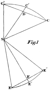
Fig. 1

Let S be the Sun (Fig. 1.), E, E′, E″, three places of the Earth, and C, C′, C″, the corresponding points in the Comet’s orbit at the three periods of observation. Join the extreme places C, C″, and E, E″, and let the intersection of the radius vector in both cases, with the chord of the arc passed over, be D and F. It is evident, that if t, t′, be the intervals of mean time between the three observations successively, t : t′ :: sector CSC′ : sector C′SC″; and in like manner, t : t′ :: sector ESE′ : sector E′SE″. If, however, we assume, for the present, that these sectors are proportional to the triangles which have as their bases the parts of the chords CC″, EE″, we shall obtain simply t : t′ :: CD : DC″ :: EF : FE″. Nor is the error of this supposition of any material consequence, in seeking the approximate elements, which is all that in the first instance we can expect. For the inequality between the ratio of the triangles (assumed proportional to the times) and the ratio of the sectors (which are truly proportional to the times), is so trifling that it is of an order higher than the sectors themselves. Besides, Newton has demonstrated that there is a certain position of the revolving radius for each parabolic or elliptic arc, which divides the chord in the exact ratio of the areas (Princip. iii. lem. 8.), and he shews that the true proportion can never differ much from the one above assumed, unless in very unequal intervals of time. With regard to the Earth, the amount of this difference is almost inappreciable, since its orbit approaches so nearly a circle. For the present, therefore, we shall assume that the chords CDC″, and EFE″ represent the observed movements of the Comet and Earth at the three periods of observation.

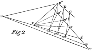
Fig. 2

Having premised these remarks, let CDC″ (Fig. 2.) be the chord in which we are to consider the motion of the Comet; and let c, d, c″, be the places in that chord projected on the ecliptic. Let S be the Sun, and E the Earth, at the time of the second observation. Join E with c″, as also with c, d, c″. Draw SE, and prolong it to cut the ecliptic in S′. Let Υ be the point on the ecliptic from which the heliocentric longitudes are reckoned; join SΥ; then EΥ′ parallel to SΥ will serve for the measurement of the geocentric longitudes.

Let L, L′, L″ = the angles S′SΥ or the arcs S′Υ, &c. viz. the longitudes of the Earth.

, ′, ″, = the angles cEΥ′, dEΥ′, ″EΥ′, viz. the geocentric longitudes of the Comet.

, ′, ″, = the angles C″Ec″, &c. viz. the geocentric latitudes of the Comet.

, ′, ″, = the straight lines Ec, Ed, Ec″, viz. the curtate distances of the Comet from the Earth.

Draw cp, dp′, c″p″ perpendicular to SES′, and join pC, p′D, p″C″; call the angles Cpc, Dp′d, C″p″c″ respectively b, b′, b″.

Then, since , and , we have . In like manner, , and . Also, , hence ; and so likewise C″p″ = .

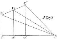
Fig. 3

Suppose that the two planes Ccp, Ddp′ are projected upon the third plane C″c″p″, (as in Fig. 3.), in which case it is evident, that CD and C″D, with all the other parts of the figure, will still bear the same proportion to one another as in Fig. 2.

Then, because sin D : Cp :: sin (b – b′) : CD, and C″p : sin D :: C″D : sin(b″ – b′), we have, by a comparison of these two series of ratios, C″p : Cp :: C″D sin (b′ – b) : CD sin (b″ – b′). Now, making the assumption (to be afterwards corrected) that the C″D, CD are exactly proportional to the intervals of time t′, t, we get C″p″ = , and substituting for C″p″, Cp their values as found above, Reducing this expression, it becomes and substituting for the values as found before, = , we obtain finally

Such is the ratio of the curtate distances of the Comet from the Earth in the first and third observations. In order to determine the real distances themselves between the Sun and Comet, join (in Fig. 2.) SC″; call SC″ = r″, and SE = R: Then, since C″p″ is perpendicular to SES′, we have C″S² = ES² + C″E² + 2SE × Ep. But EC″ = , and Ep″ = Ee″ cos C″Ep″; and therefore, since by spherics cos C″ES = cos SEc″ × cos C″Ec″ (the plane C″Ec″ being at right angles to SEc″), we have Ep″ = : Therefore, we obtain or, as we have called δ″ = Mδ, and in like manner,

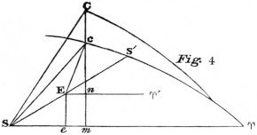
Fig. 4

We have next to determine the length of the chord CC″ joining the extreme points in which the Comet has been observed. And for this purpose, we first find the position of the comet relative to the sun, by means of the co-ordinates x, y, z. In Fig. 4. draw cm and Ee (where c is the curtate place of the Comet, E the Earth, S the Sun, and C the Comet in its orbit,) perpendicular to : Then Sm will represent x, mc = y, and Cc = z. It is evident, that , and so also ; and hence, if represent the chord between the radii vectores , , , by reduction, and substituting for their values. But we see that ; z = ; therefore, substituting, we get ; or since ,

Having thus obtained , , and , we are now to make use of them, in the following important formula where represents the time which the comet has taken to move from C to C″, and = the number ·017202, In order to demonstrate this equation, we have to compare the motion of the comet in a parabola, with some other known motion, as that of the earth. Let us for this purpose first suppose the comet’s perihelion distance to be equal to the earth’s radius vector; then, from what has been already said‍‍62, it is evident, that the velocities in the parabola and circle will be simply as , and hence the times which the comet and the earth respectively require, to pass over the same anomaly, (being inversely proportional to the velocities), will be as . Since the area of the rectangular sector in the parabola is equal to of the corresponding quadrant, we have therefore for the time which the comet will take to pass over 90° of anomaly (where A is the length of the sidereal year, and the area of a circle whose radius = ). From this we are enabled to compute the time required for describing any other angle ; for as the area = , we get area of sector 90° : area of sector :: time of describing 90° : time of describing ; and time of describing θ, which call ‍63. But as this is the time of a comet whose perihelion distance = , and as for different parabolas the times are as the powers of D their perihelion distance, we have for the time which any comet takes to describe the anomaly , . Now, if be the anomaly corresponding to the radius vector r″ at the time of the third observation, we have in like manner ; but it will be found that , since A = 365.25 = ; hence, But, by a fundamental property of the parabola, and , whence, by a mutual division, and substituting for , we have ; therefore we get finally But k being the side of a triangle opposite to the angle or 2, and r, r″ the sides adjacent, we have, by trigonometry, , and ; or, putting R for , and S for , , ; hence we find , and ; consequently, ; and by substitution, . But ; therefore , and consequently, . Now, ; so that ; and therefore . Multiplying each side of this last equation by , we have Now, if we put T, T″ for , we have, from equation (5.), seeing that The part has already been considered, let us now examine the part following . If, then, in this expression, we substitute for ″ and their values found before, , and , it becomes ; but (as above) = ; hence , so that the expression reduces itself to therefore, since it has been shewn that , we have But because ; hence, Now, , so that the two radicals in this expression are of the form , putting for . Hence, the usual rule for extracting the root of a binomial surd applies to them, the root being, as is shewn in all books of algebra, : consequently we obtain and, by reducing this equation to its simplest terms,

We have now obtained four equations (2.), (3.), (4.), (7.), comprehending the four unknown quantities , , , ; and from these we have only to extract their values. The easiest way of effecting this, in reference to these equations, is, not by resolving directly an equation of so high a power, but by the method of false position, one of the simplest and most useful rules of elimination known in mathematics. Assume some value for , as near the truth as may be conjectured, and apply this in the equations involving , in order to obtain values for , , and ; then, by substituting these values in the equation for the time, just demonstrated, call the discrepancy between the result and the known quantity . Make, then, for a new value of , some less erroneous hypothesis, ; and proceeding throughout exactly in the same manner as in the first instance, call the error this time , then , and therefore which will furnish a yet more correct value for . By substituting this corrected value of , and repeating the process a third time, we approximate still more nearly to the truth; nor is it ever necessary to resort to a sixth hypothesis, the fourth is in general sufficiently correct.

Having in this manner discovered the values of , , and , and therefore also of (which is equal to , we proceed next to extract the heliocentric latitudes and longitudes. Let represent the former, and the latter. Since , we have and (in Fig. 4.) since , we have 64 ‍

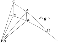
Fig. 5

From the heliocentric latitudes and longitudes, we easily obtain the place of the comet’s node, and the inclination of the orbit to the ecliptic: For in the right-angled spherical triangle (Fig. 5.), where A is the perihelion, the node, and I the angle at which the comet’s orbit is inclined to the ecliptic, we have , and ; hence , which, by a well known property of sines, gives , or 65 hence, also,

If , be the arguments of the comet’s latitude on its orbit, we have but is the same as the difference of the true anomalies, or , and therefore, we can determine the amount of each anomaly by means of the equation already demonstrated, and marked (6.) Hence, the comet’s perihelion distance, is obtained, and the longitude of the perihelion, not reduced to the ecliptic, from the equation Finally, we derive the time of the perihelion passage before the first observation, from the formula demonstrated on page 63.,66 ‍ The perihelion passage will be before or after the first observation (in the case of direct motion), according as the longitude π of the perihelion is less or greater than the heliocentric longitude l at the first observation; the reverse will be the case in retrograde motion.

The method which we have now demonstrated, of discovering from three observations of a comet, what are the elements of its orbit, is allowed to be one of the simplest and most convenient known to astronomers. After having obtained the geocentric latitudes and longitudes of the comet, we can in the course of a few hours labour, obtain a near approximation to its place and path in the system. But simplicity of solution, and facility of calculation, are not the only advantages which distinguish the method of Olbers. It is found also to represent with accuracy the motion of comets in general, and of all those especially whose orbits, from their great eccentricity do not differ much from a parabola.

We proceed to show the application of these formulæ, by employing them in the investigation of the orbit of a particular comet. The Comet observed at Paramatta in 1826, having been proposed for that purpose, the following are the observations of it made by Mr Rumker, as given in the Philosophical Magazine April 1827.

Paramatta, Sidereal Time. h ′ ″ 1826, Sept. 4. at 4 19 19 6. ... 2 23 9 7. ... 3 44 20 8. ... 2 4 25 9. ... 3 19 0 Right Ascension. ° ′ ″ 84 13 47 87 27 35 89 13 47 90 48 44 92 37 20 Declination. ° ′ ″ -8 49 0 -6 53 43 -5 49 8 -4 49 15 -3 39 7

Since in the foregoing method three observations only are necessary, we fix upon the first, second, and fourth, as affording intervals of time the least unequal. The first step is to extract from these data the geocentric longitudes and latitudes of the comet, as well as the mean solar time at Greenwich. The longitude of Paramatta is 10° 4′ 14″.5 East of Greenwich.

Mean Solar Time at Greenwich. h ′ ″ Sept. 4. at 7 21 35 = 4·306656 6. ... 6 17 52 = 6·220741 8. ... 4 51 19 = 8·202309 Comet’s Longitude. ° ′ ″ 83 15 42 87 4 40 90 53 53 Comet’s Latitude. ° ′ ″ -32 8 33 -30 19 49 -28 16 45‍‍67

The apparent motion of the Comet being determined, we have next to find the position of the Earth at the several periods, by means of the sun’s longitude and the earth’s radius vector. These are found to be,

161° 40′ 2″ 163° 31′ 35″ 165° 27′ 10″

1·0077198 1·0072182 1·0066872

Several small corrections, however, must be applied, before these data can represent accurately the comet’s route in the heavens. It is presumed that the errors of Refraction have been already expunged: it only remains to calculate the effects of Precession, Aberration, Nutation, and Parallax.

Let the epoch from which the apparent places are to be computed be the 1st January 1827. The Precession for the first observation is ; for the second, ; and for the third, .

In the Nautical Almanack, we find the Nutation to be -15′.1, -15″.1, -15″: it is taken with the sign reversed, as the observed or apparent positions must be converted into the mean.

In order to estimate completely the Aberration, we ought to know the distance of the Comet from the Earth. But as this is as yet unknown, we must proceed according to the method pointed out by Gauss, (70.) by first correcting the latitudes and longitudes of the comet for the aberration of fixed stars, and afterwards applying the requisite correction when the above element is determined.

The aberrations of the stars is thus found by the table (Encycl. Edin. p. 801.),

The ☉’s longitude, 161° 40′

Comet’s longitude, 83 16

78 24 gives 4″.02

Comet’s latitude, 32 8 sec. of 1 .18

Aberration in longitude for first observation, = 4 .7

which must be applied with the contrary sign, for the same reason as in the case of nutation; so also 5″.4, and 6″ are the aberrations for the other two observations. The aberrations in latitude are -10″.4, -9″.8, and -9″.

Comet’s longitude, 83° 15′ 42″ 87° 4′ 40″ 90° 53′ 53″

Precession, +16.2 +15.9 +15.6

Aberration, + 4.7 + 5.4 + 6

Nutation, -15.1 -15.1 -15

Corrected longitude, 83° 15′ 47″.8 87° 4′ 46″.2 90° 53′ 59″.6

Comet’s latitude, -32° 8′ 33″ -30° 19′ 49″ -28° 16′ 45″

Aberration, -10.4 - 9.8 - 9

Corrected latitude, -32 8 43 .4 -30 19 58 .8 -28 16 54

The positions of the Earth must be freed also from the effect of Parallax.

Parallax‍‍68, -6″.8 -6″.9 -7″

Precession, +16.2 +15.9 +15.6

Aberration for sun, +20 +20 +20

Nutation, -15.1 -15.1 -15

Earth’s longitudes, 341° 40′ 2″ 343° 31′ 35″ 345° 27′ 10″

Corrected longitudes, 341 40 16 .3 343 31 48 .9 345 27 23 .6

Radii vectores, 1·007719 1·007218 1·006687

Parallax, + 000019 + 000036 + 000041

Corrected Radii, 1·007739 1·007254 1·006728

Mean Time. Comet’s Longitudes. Comet’s Latitudes. Earth’s Longitudes.

° ′ ″ ° ′ ″ ° ′ ″

1826, Sept. 4.306656 λ = 83 15 48 β = -32 8 43 L = 341 40 16

6.220741 λ′ = 87 4 46 β′ = -30 19 59 L′ = 343 31 49

8.202309 λ″ = 90 53 59 β″ = -28 16 54 L″ = 345 27 24

t = 1·914085, t′ = 1·981568, R = 1·007739, R′ = 1·007254, R″ = 1·006728.

We now proceed to apply these values in the formulæ already demonstrated. In the first place, we compute by means of the equation69

‍‍

log sin(L′- λ′) = 256° 27′ 2″ = 9·9877414 - log sin(L′ - λ″) = 252° 37′ 49″ = 9·9797296 -

log tan β = 32 8 43 = 9·7982366 - log tan β′ = 30 19 59 = 9·7672501 -

·61091114 = 9·7859780 + ·55844412 = 9·7469797 +

log sin(L′ - λ) = 260° 16′ 0″ = 9·9937030 - log sin(L′ - λ′) = 256° 27′ 2″ = 9·9877414 -

log tan β′ = 30 19 59 = 9·7672501 - log tan β″ = 28 16 54 = 9·7308080 -

·57670414 = 9·7609531 + ·52305748 = 9·7185494 +

Numerator, ·03420700 = 8·5341150 ·03538664 Denominator.

Denominator, ·03538664 = 8·5488393 log t′ = 1·981568 = 0·2970089

9·9852757 log t = 1·914085 = 0·2819611

= 0·0150478 ............................... 10·0150478

0·0003235 = log M.

Having thus obtained M, we employ it to find the comet’s distance from the sun, at the first and third observations, in the formulæ (2.) and (3.).

° ′ ″ ° ′ ″

log sec β = 32 8 48 = 0·0722696 log sec² β″ = 28 16 54 = 0·1104140

× 2 log M² = 0·0006470

sec² β = 1·39488738 = 0·1445392 1·29140059 = 0·1110610

° ′ ″ ° ′ ″

log = cos(L - λ) = 258 24 27 = 9·3030873 - log cos(L″ - λ″) = 254 33 24 = 9·4253470 -

log R = 1·007739 = 0·0033481 log R″ = 1·006728 = 0·0029122

log 2 = 0·3010300 log 2M = 0·3013535

- ·405009746 = 9.6074654 - - ·536553125 = 9·7296127

log R = 1·007739 = 0·0033481 log R″ = 1·006728 = 0·0029122

R² = 1·01553818 = 0·0066962

R″² = 1·0135014 = 0·0058244

= 1·01553818 + 1·39488738 - ·405009746

= 1·01350140 + 1·29140059 - ·536553125

= 2·02903958 + 2·68628797 - ·941562871

We next calculate the chord joining the two extreme positions of the comet by means of equation (4.)

° ′ ″ ° ′ ″

log tan β″ = 28 16 54 = 9·7308080 - log cos (L - λ″) = 250 46 16 = 9·5176481 -

log tan β = 32 8 43 = 9·7982366 - log 2MR = 0·3047016

·33809954 = 9·5290446 + - ·66427776 = 9·8223497 -

° ′ ″ ° ′ ″

cos (λ″ - λ) = ·99113144 = 7 38 11 log cos (L″ - λ) = 262 11 35 = 9·1330138 -

1·32923098 = 0·1236004 log 2R″ 0·3039422

log 2M = 0·3013535 - ·27349912 = 9·4369560 -

+ 2·66044242 = 0·4249539 - ·93777688

° ′ ″

2·02903958 + 2·68628797δ² - ·94156287δ cos (L″ - L) = 3 47 8 = 9·9990514

2·02461137 - 2·66044242δ² + ·93777688δ log 2RR″ = 0·3072903

k²= ·00442821 + ·02584555δ² - ·00378598δ + 2·02461137 = 0·3063417

We have now to compute from these three equations the values for r, r″, and k. The formula supplies the fourth equation necessary for the elimination of these unknown quantities, T being in the present case 3·895653 days. As it is not practicable to resolve these equations directly, let us apply the method of false position, by assuming different hypotheses for .

In the first place, let us assume = 1. In this case, we find

r² = 1·01553818 + 1·39488738 - ·40500975 = 2·0054158 and log r = 0·1511022

r″² = 1·01350140 + 1·29140059 - ·53655312 = 1·7683488 ... log r″ = 0·1237839

k² = ·00442821 + ·02584555 - ·00378598 = ·02658777 ... log k = 2·2123409

r = 1·416127, r″ = 1·329792, k = 0·16305

(r + r″ + k)-(r + r″ - k)=·81048, log = 9·9087423

9·0137302

10·8950121 =7·8526 days

The result ought to have been 3·8956 = t + t′, rather less than half. Let us for a second hypothesis take = ·5. In this case we get

r² = 1·015538 + ·348722 - ·202505 = 1·161755, and log r = 0·0325573

r″² = 1·013501 + ·322850 - ·268276 = 1·068075, ... log r″ = 0·0143009

k² = ·004428 + ·006461 - ·001893 = ·0091962, ... log k = 2·9818042

r = 1·077847, r″ = 1·033477, k = ·095897,

(r + r″ + k)-(r + r″ - k) = ·417990 log = 9·6211659

9·0137302 3·89565 = T

0·6074357 = 4·04982 days

+ ·15417 Error

The value assumed for is yet too large, though evidently not very distant from the truth. To find a more correct hypothesis, we employ the method already pointed out (8.), . Let us then calculate the equations on this third hypothesis:

r² = 1·0155381 + ·3213820 - ·1944046 = 1·14251555, log r = 0·0289310

r″² = 1·0135014 + ·2975387 - ·2575455 = 1·05349460, log r″ = 0·0113161

k² = ·0044282 + ·0059548 - ·0018172 = ·00856579, log k = 2·9663837

r = 1.068885, r″ = 1.026398, k = .092551,

(r + r″ + k)-(r + r″ - k) = ·401873, log = 9·6040888

log 6μ = 9·0137302 3·89565 = T

0·5903586 = 3.89366 days

- ·00199 Error.

It is evident that we have assumed the value of rather too small. Let us next try ·48037:

r² = 1·01553818 + ·32187773 - ·19455449 = 1·14286142, log r = 0·0289967

r″² = 1·01350140 + ·29799761 - ·25774400 = 1·05375501, log r″ = 0·0113698

k² = ·00442821 + ·00596400 - ·00181867 = ·00857354, log k = 2·9665801

r = 1·06904688, r″ = 1·02652542, k = ·09259342,

(r + r″ + k)-(r + r″ - k) = ·4020855, log = 9·6043184

log 6μ = 9·0137302 3·895653 = T

0·5905882 = 3·895724 days

+ ·000071 Error.

The aberration from the truth is now very trivial; let us, however, make a fifth hypothesis, and call = ·4803483 as derived from a comparison of the two last, we then find,

r² = 1·01553818 + ·32184873 - ·19454572 = 1·14284119, and log r = 0·0289929

r″² = 1·01350140 + ·29797075 - ·25773236 = 1·05373979, ... log r″ = 0·0113667

k² = ·00442821 + ·00596346 - ·00181859 = ·00857308, ... log k = 2·9665684

r = 1·06903739, r″ = 1·02651828, k = ·09259092,

(r + r″ + k)-(r + r″ - k) = ·402071, log = 9·6043028

log 6μ = 9·0137302 3·895653 = T

0·05905726 = 3·895584 days

- ·000069 Error.

The true value of lies therefore between ·48037 and ·4803483. It will be sufficiently accurate to institute the following proportion:

Fourth hypothesis, = ·48037 r = 1·06904688 r″ = 1·02652542, T = 3·895724

Fifth hypothesis, = ·4803483 = 1·06903739 = 1·02651828, = 3·895584

·0000217 ·00000949 ·00000714 ·000140

Diff. Error. Diff. Error.

·000140 : ·000069 :: ·0000217 : ·0000107, hence = ·4803590 log = 9·6815659

·00000949 : ·00000467, r = 1·0690406 log M = 0·0003235

·00000714 : ·00000352, r″ = 1·0265280 log ″ = 9·6818894

Having thus determined the comet’s distances from the sun, at the first and third observations, together with its curtate distances from the earth, we next proceed to determine the heliocentric latitudes and longitudes, as well as the elements of the orbit. From the diminution of the radius vector, it is evident that the comet was at this time approaching its perihelion.

are the formulæ.

° ′ ″ ° ′ ″

log tan β = 32 8 43 = 9·7982366 log tan β″ = 28 16 54 = 9·7308080

log δ = 4803590 = 9·6815659 log δ″ = ·4800714 = 9·6818894

9·4798025 9·4226974

log r = 1·0690420 = 0·0289947 log r″ = 1·0265218 = 0·0113682

sin b = 16 24 4.5 = 9·4508078 sin b″ = 14 35 36.5 = 9·4013292

° ′ ″ ° ′ ″

sin (L - λ) = 258 24 27 = 9·9910495 - sin (L″ - λ″) = 254 23 24 = 9·9840294 -

log δ = ·4803590 = 9·6815659 log δ″ = ·4800714 = 9·6818894

9·6726154 - 9·6659188 -

° ′ ″ ° ′ ″

log cos b = 16 24 4.5 = 9·9819580 log cos b″ = 14 35 36.5 = 9·9857578

log r = 1·0690420 = 0·0289947 log r″ = 1·0265218 = 0·0113682

10·0109527 9·9971260

° ′ ″ ° ′ ″

sin (L - l) = -27 18 44.3 = 9·6616627 - sin (L″- l″) = -27 48 11.7 = 9·6687928 -

L = 341 40 15.2 L″ = 345 27 28

sin l = 8 58 59.5 sin l″ = 13 15 34.7

Having thus computed the heliocentric latitudes and longitudes, we next find the place of the Node, which, in the case of direct motion, will be the comet’s ascending node. The increase of the longitudes, shows that this comet is direct, and the diminution of the latitudes, which are south, that it was situated in the part of its orbit below the ecliptic, and moving towards the point of intersection. The place of the Node may be computed by means of the formula, 70.

° ′ ″ ° ′ ″

log tan b = 16 24 4.5 = 9·4688488 log tan b = 16 24 4.5 = 9·4688488

log sin l″ = 13 15 35 = 9·3605282 log cos l″ = 13 15 35 = 9·9882647

·067511376 = 8·8293770 ·286492659 = 9·4571135

log tan b″ = 14 35 36.5 = 9·4155723 log tan b″ = 14 35 36.5 = 9·4155723

log sin l = 8 58 59.5 = 9·1935274 log cos l = 5 58 59.5 = 9·9946401

·040653665 = 8·6090997 ·257165294 = 9·4102124

Numerator = ·026857711 = 8·4290690 ·29327365 Denominator.

Denominator = ·029327365 = 8·4672729

9·9617961 = 42° 28′ 56″.3 = tan Ω.

By equation (12.), we find the inclination of the comet’s orbit to the ecliptic‍‍71: and by equation (13.), , the arguments of the latitude‍‍72.

° ′ ″ ° ′ ″

log cos b = 16 24 4.5 = 9·9211070 log cos b″ = 14 35 36.5 = 9·9857577

log cos (l - Ω) = 33 29 59.7 = 9·9819580 log cos (l″ - Ω) = 29 13 24.2 = 9·9408764

cos u = 36 52 27.2 = 9·9030650 cos u″ = 32 22 27.9 = 9·9266341

log tan b = 16 24 4.5 = 9·4688488 u = 36 52 27.2

log sin (l - Ω) = 33 29 59.7 = 9·7418885 u - u″ = 4 29 59.3

tan I = 28 4 13.3 = 9·7269603 (u - u″) = 2 14 59.6

Having thus obtained the arguments of the latitudes, whose difference is the same as that of the true anomalies, we are enabled to calculate the anomaly itself at the first observation by the equation‍73

‍

° ′ ″

= 2 14 59.6 = 9·9996650 = ·99922902 log = 10·0289947

log = 10·0113682

= 0·0088132 = 1·02050047 log = 10·0176265

° ′ ″

8·3277971 = 0·2127145 = 56 54 3.2

= 2 14 59.6 = 1·4060705 = 4 29 59.3

tan = 28 27 1.6 = 9·7338676 ″ = 52 24 3.9

The Perihelion Distance, and longitude of the Perihelion, are derived from the equations ⁠74, and .

° ′ ″ ° ′ ″

log cos = 28 27 1.6 = 9·9441023 = 56 54 3.2

2 u = 36 52 27.2

log cos² = 9·8882046 - u = 20 1 36

log r = 0·0289947 Ω = 42 28 59.2

D = ·8264172 = 9·9171993 π = 62 30 35.2

It only remains to calculate the time of the Perihelion Passage, which must evidently be posterior to the last observation, since the longitude of the perihelion is greater than the comet’s heliocentric longitude. The anomaly at last observation having been 52° 24′ 18″.9, we look in the table for the number of days corresponding.

Opposite to 52° 12′ 9″.8 is 43.50 days, and the difference between this anomaly and

the comet’s, viz. 11 54 .1 gives .21923 for the corresponding interval: therefore,

the anomaly, 52 24 3 .9 gives 43.71923, log = 1·6406725

log D = 9·8757989 = 8·202309 time of 3d obs.

1·5164714 = 32·845160 days.

Perihelion Passage = 41·047469 days subsequent

to the 1st September‍‍75.

The approximative elements of this comet, obtained by the foregoing investigations, are therefore,

Greenwich.

Passage of Perihelion, 1826, Oct. 11·047468

Longitude of Perihelion, 62° 30′ 35″

Longitude of the Node, 42 28 59

Inclination of Orbit, 28 4 13

Distance of Perihelion, ·8264172

Motion, Direct.

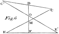
Fig. 6

Still, it must be remembered, that the elements, as thus obtained by Olbers’ method, on account of the imperfection of the method, are no more than approximate. One of the fundamental data on which that method is grounded, however slight its aberration from the truth, is nevertheless not mathematically correct. It will be recollected, that, at the commencement of the method, we assumed that the radii vectores of the earth and of the comet divide the chords of the arcs passed over by them, in the exact proportion of the times;—an assumption involving a slight inaccuracy, but which served to facilitate considerably the solution of the problem. We have now therefore to rectify the value of ″, as given by equation (1.) and, instead of supposing it = M, let us make it = (M + v) + h. We have only to determine v and h, to find the real value of ″. It is evident from Fig. 1. that EF : FE″ :: SE × sin ESF : SE″ × sin FSE″; and in like manner, that CD : DC″ :: SC × sin CSD : SC″ × DSC″. It is also evident, that the angles ESF, FSE″, are the differences between the earth’s longitudes, in the second and third observations; and that the angles CSD, DSC″, are the differences between the comet’s true anomalies, also in the second and third observations, determined by the foregoing investigations: So that calling these last angles τ and σ, we obtain from the above proportions , and . In the accompanying figure, let CDC″, EFE″ be the chords of the comet and of the earth, projected on a plane perpendicular to the intermediate radius vector of the earth, or a circle of latitude. Join the intermediate points D F, by the line DF, cutting C″E″, CE, in O and M. Now, since C″O : sin D :: C″D : sin O, by the common property of triangles, and sin D : CM :: sin M : CD. Therefore, we obtain by the comparison of these two series,

C″O : CM :: C″D × sin M : CD × sin O.

In the same manner, we get

E″O : EM :: E″F × sin M : EF × sin O:

from both of which we obtain Now, calling EM, ; and EC, , we have CM = . We have likewise, as at the commencement of the parabolic investigation, M, (or the angle at the intersection of the first and second projected distances, EC, FD) = : and D (or angle formed by the second and third projected distances) = : so that, making these substitutions, the above equation becomes

If now we put , and , we have, from equations (16.) and (17.) the first being the correction for the comet’s orbit, the other for the earth’s. But so that calling , we get Now, in deducing equation (1.) we found C, or (since E is here supposed projected on the plane C), , and or whence we now have If in this last, and somewhat complicated equation, m is substituted for , we obtain So that this last term of the equation becomes this expression may be converted also into76 The whole equation becomes therefore

With this corrected value for the ratio of , we may proceed at once to amend our calculations. But, as Olbers observes, the labour is much abridged, by recollecting that the already computed can differ very slightly from the true value now to be found; and if we call the approximate value (), we shall have , and the above equation for becomes being = . In order, therefore, to correct the equations (2.) and (7.), giving the approximate values of ″ and , we must multiply all the coefficients which contain M, by , and those containing by . The equation for remains of course unaltered, as M does not enter into any of its terms.

For the sake of conveniently applying the equations requisite for determining H, let us collect them from the preceding investigations. Having already obtained the approximate values of σ, τ, and ″, we have only to substitute them, along with that of , in the following equations. where, as before, and finally, for, in the last term of the equation for H, the quantities h and M have the same denominator, which necessarily disappears in the fraction .

This method of correction just demonstrated, is very simple, and equally convenient for calculation. It is also, in its application, extremely general; for, by means of it, we are enabled to amend the approximate elements, without being obliged to resort to any other observations than the three, if they are not remote from one another, which have been already employed in obtaining them. But it is to be remarked, that the orbit of a comet will be determined much more correctly, if the observations are made after the lapse of considerable intervals; because then the small errors committed either in observation or computation, or which arise from inaccuracies in the sun’s tables themselves, when thus diffused over a considerable space, have that influence lessened which otherwise would affect the correctness of the results. It is therefore extremely desirable, when we happen to possess a long series of observations, comprehending, for instance, intervals of twelve or sixteen days, to be able to employ them in a more complete rectification of our approximate elements; and the ingenuity of Olbers has here also supplied a method alike remarkable for its conciseness and certainty.

Fix upon two extreme observations, as far distant as possible from each other, and, by means of the elements already computed, determine the curtate distances Δ Δ″ of the comet from the sun, and likewise the heliocentric latitudes and longitudes. These computations are readily made; for the angle at the projected place of the comet on the plane of the ecliptic (Fig. 4.) is found by the equation observing, however, to take the angle acute or obtuse, according to circumstances; and hence we find , the elongation of the comet from the earth = : and for the heliocentric latitude, since we have the equation The heliocentric longitudes may then be obtained by means of equat. (10.), We then make successively two small variations in the curtate distances, Δ + m, and Δ″ + n; and the hypotheses will stand thus:

1st Obs............. Δ, Δ + m, Δ

3d Obs. ............ Δ″, Δ″, Δ″ + n.

According to the method already pointed out, we next compute the longitude of the ascending node, and the inclination of the orbit for each of these three hypotheses; and since , and , we hence find the anomalies in both observations, the distance of the perihelium, and the time from the perihelium to the first and third observations, which gives us the time that ought to elapse between these observations, according to each of the hypotheses; hence we have the first comparison. We then add, for each of the three orbits, to the time between the perihelium and the first observation, the observed time from the first to some other observation, sufficiently remote from both the others: Lastly, we compute the geocentric place of the comet, in longitude or latitude, according as the one or other varies most rapidly, and the place so computed gives, together with the observation, the second comparison.

The whole proceeding will ultimately stand thus:

1st Hyp. 2d Hyp. 3d Hyp. True Orbit.

Curtate distance, 1st observation, Δ Δ + m Δ Δ + x

..... ..... 3d observation, Δ″ Δ″ Δ″ + n Δ + y

Time between 1st and 3d observ. τ τ + p τ + q T observ.

Longitude in 2d observation, a′ a′ + r a′ + s λ′ observ.

By the method of false position, we obtain from the comparison of these true and hypothetical values, from which equations we obtain finally‍77

As an example of the manner of rectifying the approximate parabolic elements of a comet, let us take the same comet observed at Paramatta, whose orbit has been already calculated. In choosing which method of correction we shall employ, it may be noticed, that, in this example, there are no observations comprehending any considerable intervals of time; and therefore, we must resort to the first of the two methods pointed out.

Recollecting, then, the quantities which enter the formulæ, we have to compute, in the first place, the comet’s anomaly at the second observation, in order to find the values of and .

We have already found, that the Perihelion Passage took place 41·047469 days after the 1st September, whence 34·826728 is the interval between the perihelion passage and the second observation, which corresponding to 54° 44′ 8″.1 of anomaly; and hence = 2° 20′ 4″.2, and =2° 9′ 55″.1.

° ′ ″ ° ′ ″

log sin σ = 2 20 4.2 = 8·6099510 log sin (L″ - L′) = 1 55 35 = 8·5265395

log r″ = 0·0113682 log R″ = 0·0029122

8·6213192 8·5294517

log sin τ = 2 9 55.1 = 8·5772932 log sin (L′ - L)) = 1 51 33 = 8·5111195

log r = 0·0289947 log R = 0·0033481

8·6062879 8·5144676

1·03521669 = 0·0150313 1·03510428 = 0·0149841

In order to find q and p, we ought now to subtract from these values , but as in the commencement of the process we deferred applying the full correction for aberration, until the comet’s distance from the earth had been ascertained, we have now to make a small alteration in the intervals. We have already found the comet’s curtate distance at the first and third observations. The real distance is equal to , and we have to multiply it by 493″, or ^D0·005706.

log δ = 9·6815659 log δ″ = 9·6818894

log cos β = 9·9277304 log cos β″ = 9·9447930

9·7538355 = log comet’s dist. 9·7370964 = log comet’s dist.

7·7563318 = log 0·005706 7·7563318 = log 0·005706

log Reduct. = 7·5101665 = ·003237 log Reduct. = 7·4934282 = ·003115

Time of 1st obs. = 4·306656 Time of 3d obs. = 8·202309

Corrected, 4·303419 Corrected, 8·199194

In order to find the correction for the second observation, the comet’s distance must be calculated by means of the elements already obtained. We find ′ by means of the equation ′ = , the log. of which is 10·0213005, and ′ = 34° 42′ 32″·1. The comet’s real distance from the earth = , whence is found

log comet’s dist. = 9·7458053

log 0·005706 = 7·7563318

log Reduction = 7·502137 = ·003177

Time of 2d obs. = 6·220741

Corrected, = 6·217564

Whence the intervals now are t = 1·914145, and t′= 1·981630.

log ′ = 0·2970226

log = 0·2819748 1·03521669 1·03510428

log = 0·0150478 = 1·03525595 ............ 1·03525595

5·5939503 = -·00003926 = -·00015167 =

log = 9·9849522 -·00003926 =

= 5·5789025 = -·000037923 -·00011241 =

log = 8·5144676 log tan β′ = 30° 19′ 59″ = 9·7672501 -

log = 6·0507663 - sin = 103 32 58 = 9·9877414

log = 9·7795087 - log = 9·7795087 -

4·3447426 + sin = 99° 44′ 0″ = 9·9937030

log = 8·5463718 -·59321441 = 9·7732117 -

log = 9·6815659 +·62840057 = -tan β

log = 0·0150478 +·03518616 = 8·5463718

8·2429855

log = 6·1017571 =1·000126403 = 1 +

− ·000037923 =

H =1·00008848 and log H = 0·00003842

With this correction we proceed to rectify the value of M, found at the commencement of the calculation. The equations for ″and will accordingly suffer some alteration, in the terms which involve M. These terms must be multiplied by H when they contain M, and by H² when M² occurs; the equation for r remains the same. We then find

= 1·01350140 + 1·29162921 - ·53660049 corrected.

= 1·01553818 + 1·39480738 - ·40500974 as before.

= 2·02903958 + 2·68643659 - ·94161023

2·02461137 - 2·66067800 + ·93783558

= ·00442821 + ·02575859 - ·00377465

With these new equations, which do not differ much from those formerly obtained, we proceed to find the correct value of . Let us as our first hypothesis take = ·48037 as before. In this case,

r² = 1·01553818 + ·32187773 - ·19455449 = 1·14286142, log r = 0·0289967

r″² = 1·01350140 + ·29798554 - ·25773883 = 1·05374811, log r″ = 0·0113760

k² = ·00442821 + ·00596422 - ·00182255 = ·00856988, log k = 2·9664874

r + r″ + k = 2·18810147, r + r″ - k = 2·00307275, (r + r″ + k) - (r + r″ - k) = ·4017436

whence ·4017436/6 = 3·892411, which, subtracted from t + t′ = 3·895775, leaves -·003364 as the error. As a second hypothesis, let be assumed = ·48099. We then find,

r = 1·0693181, r″ = 1·0267528, k = ·0925846, and (r + r″ + k) - (r + r″ - k) = ·4020942,

which, divided by 6μ, gives 3·895807, the error of which is only +·000032. Comparing now these two hypotheses, the method of false position gives ·480984 as a more correct value. Proceeding on this third assumption, we get

r = 1·06931394, r″ = 1·02675071, and k = ·09258402, (r + r″ + k) - (r + r″ - k) = ·4020911,

which gives 3·895779 days as the result, the error now being only -·000004. The last hypothesis, therefore, may be taken as the value of . In order to find ″, we must add to log δ the logarithms of M and of H, which gives ″ = 9·6824918.

In the same manner, exactly as before, we calculate, by means of these data, the heliocentric elements. The latitudes b and b″ are found to be respectively 16° 25′ 8″, and 14° 36′ 39″: the longitudes l and l″ 9° 1′ 0″.7, and 13° 17′ 50″. The longitude of the node is 42° 33′ 48″.7, and the inclination of the orbit 28° 4′ 5″.2. The arguments of the latitude at the two periods are u = 36° 55′ 21″, and u″ = 32° 25′ 10″, from which the comet’s anomaly is found to be θ = 56° 54′ 18″, and θ″ = 52° 24′ 7″. The perihelion passage is thence found to be 41·059761 days after the first observation, and the corrected elements are as follows‍‍78:

Mean Solar Time at Greenwich.

Perihelion Passage, 1826, October 11·059761

Longitude of the Perihelion, 62° 32′ 46″

Longitude of Ascending Node, 42 33 49

Inclination of the Orbit, 28 4 5

Perihelion Distance, ·8265950

Motion, Direct.

VI. Such is the method by which the Parabolic elements of a comet’s orbit may be determined. Those elements are always sought by astronomers first, on account of the comparative facility with which they may be calculated, and the sufficient degree of correctness with which they represent the movements of any particular comet.

The period of the comet’s revolution is an element concerning which the Parabolic method necessarily can afford no intelligence. It is calculated to point out the course of the comet, only while it remains in the vicinity of the earth, and cannot follow it in its eccentric track through the whole system. But if the parabolic hypothesis is therefore not so perfect as to point out immediately the comet’s period of revolution, there is an indirect method by means of which, with these elements alone, it is possible to discover this important element, with perhaps even greater certainty than by the elliptic hypothesis. With the parabolic elements we search among all the comets formerly observed, if there are any which agree; and if in this manner two comets are found possessing elements nearly the same, then there is a high degree of probability that the two comets are identical; and the probability will be increased, if there be a third or a fourth comet with similar elements, and which passed the perihelion at about the same interval of time as the former. The data on which we are to proceed in the comparison, are, the perihelion distance, the position of the perihelion, the place of the nodes, and the inclination of the orbit to the ecliptic. If these elements differ only very little from one another, in the case of two or more comets, it is extremely probable that they will turn out to be the same one which has been observed at its successive returns to the sun. It was by this method that Halley first ascertained the period of the Comet seen in 1682, and which he predicted would again appear in 1759. He observed that its elements agreed very nearly with those of the comets which had been seen in the years 1607, 1531, and 1456, between each of which there was an equal interval of seventy-five or seventy-six years‍‍79. According to this estimate, it ought also to have come to its perihelion in the years 1380, 1305, and 1230; and it so happens that historians speak of a remarkable comet which was observed in each of those several years. This comet did appear, as Halley had announced, in 1759, though its period was made somewhat longer by the attraction of Jupiter and Saturn. On the same data, there is not the least doubt that this comet will again reach its perihelion about the year 1834.

But astronomers are not satisfied with this indirect and retrospective method of ascertaining the periodic revolutions of comets, for which a succession of many ages often is required. They must possess a method more immediate—a method by which, from three present observations, without reference to the history of former comets, they can at once say when a comet now seen for the first time last passed its perihelium, and when it will again become visible. Moreover, it is found, that there are some comets whose course through the heavens cannot be correctly represented by any Parabola; because, when the true orbit is not very elongated, it will differ from that curve even towards the vertex; and this aberration occasions considerable errors in the elements themselves. It is therefore in some cases desirable to determine the movement of the comet through the system on more accurate data; and this object, as well as the immediate determination of the periodic time, is attained by computing the Elliptic elements.

Of the various solutions which have been given of this difficult problem, none seem to be so generally recommended and resorted to by astronomers as that of Gauss. La Place may have displayed greater dexterity in managing the powers of the higher calculus—many mathematicians may have proposed other solutions better adapted to particular circumstances—but Gauss’s method can be much more readily employed in practice, and is found to apply to every possible case. I now therefore proceed to point out the manner in which, according to Gauss’s method, the Elliptic elements of a comet’s orbit may be found.

But it is quite impossible here to do more than merely develope the mode of procedure, in so far as may be necessary for calculation; because, were I to detail each step in the complicated investigation, as I have been led to do in the shorter method of the parabola, it would require us to enter on a long train of analytical reasoning, quite inconsistent with the due limits of this Essay. I am under the necessity, therefore, of giving only those equations which are immediately subservient to the actual computation of the elements, shortly describing, however, the process by which the greatest part of them is derived; and in the rest, where the demonstration is too tedious to be pointed out, referring to Gauss’s great work “Theoria motuum corporum cœlestium.” The same method is also demonstrated at great length in one of the volumes of Delambre’s Astronomy, where the whole investigations of the formulæ are minutely detailed, and where, at the same time, various examples are given of their application. I may remark generally, that there are certain leading features common to both methods, by which the procedure in the method now to be pointed out is very similar to the parabolic hypothesis. The only difference arises from the peculiar nature of the curves, by which the elliptic method is rendered more involved, but is not dissimilar in general character.

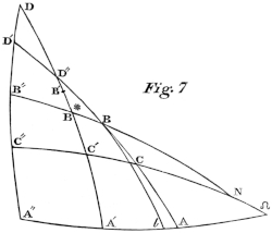
Fig. 7

Let A, A′, A″ (Fig. 7.) be the heliocentric places of the earth at the three periods of observation, and B, B′, B″ the geocentric places of the comet. Let great circles pass through these points, joining AB, A′B′ and A″B″. The first object is to determine the position of these circles with respect to the ecliptic AA″, as well as the position of the points B, B′, B″. For this purpose, let the angles which these great circles make with the ecliptic be called y, y′, y″‍‍80, and the arcs themselves AB, &c. , ′, ″: then, denoting, as before, the geocentric longitudes of the comet by , ′, ″, its geocentric latitudes by , ′, ″, and the heliocentric longitudes of the earth by L, L′, L″; it is obvious, by drawing a perpendicular to the ecliptic from B, that‍81 In the same manner, y′, y″, and δ′, δ″ are computed.

In order now to estimate the position of the great circles AB, &c. with respect to one another, let them intersect in the points D, D′, D″, and call the angles at these points respectively ε, ε′, ε″. In the spherical triangle A′DA″, it may be shown that

sin ε sin (A′D + A″D) = sin (L″ - L′) sin (y″ + y′),

sin ε cos (A′D + A″D) = cos (L″ - L′) sin (y″ - y′),

cos ε sin (A′D - A″D) = sin (L″ - L′) cos (y″ + y′),

cos ε cos (A′D - A″D) = cos (L″ - L′) cos (y″ - y′),

in which equations sin ε, and cos ε are always positive. From them we extract the values of A′D, A″D, and ε. By considering in like manner the other two triangles, we obtain AD′, A″D′, ε′, and AD″, A′D″, ε″‍‍82.

Let the two extreme geocentric places B, B″ of the comet be now joined by a great circle, in the same manner as in the parabolic method. This great circle must intersect A′B″, but will probably not pass through B′, the second place of the comet. Call the distance of the intersection from B′ or B′B* = ; and we then obtain finally an equation, which combines the respective positions of the earth and comet,

We now pass from the geocentric to the heliocentric situation of the Comet. Let C, C′, C″ be its three places, as seen from the sun: these points will lie somewhere in the corresponding great circles AB, A′B′, A″B″, and at the same time be united by another great circle, viz. that which forms the projection of the orbit on the celestial sphere. Preserving the same notation as before, let the radius vector of the comet at its several places be r, r′, r″, and the corresponding radius vector of the earth R, R′, R″. Now, it is a property of the ellipse, that if η represent a sector bounded by the two radii vectores r, r″ and the intervening curve 2h, t the time which is required to describe this sector, and a constant number ·017202 (employed also in the parabolic investigation), the semi-parameter = Make , which is the triangular sector = ; and ; then the semi-parameter is equal to Let ; and , where ′ is the sector formed by , ″ and the chord of 2′. But as , ′ ″; , ′ ″ and therefore , ″ are yet unknown, let us for the present assume , and . Find next the value of the equations‍‍83 , , . Then we get , and , where represents the arc C′B′‍‍84.

We next compute the two equations , and , from which we get , and

The following four equations , , , enable us to calculate , . From these we obtain , ″, , ″ by the equations

If now C′C″, CC″, CC′, or the differences of the comet’s heliocentric longitudes on its orbit, be represented by 2, 2, 2, and ″, be the inclinations of the great circles AB, A″B″ to the great circle CC″, we shall have the following four equations for the determination of ′, as well as of ″ and :

sin f′ sin (k″ + k) = sin ′ sin ( + ″)

sin f′ cos (k″ + k) = cos ′ sin (′ - ″)

cos f′ sin (k″ - k) = sin ′ cos ( + ″)

sin f′ cos (k″ - k) = cos ′ cos ( - ″)

The two first of these give (k″ + k), and sin f′, and the two others (k″ - k), and cos f′. At present, however, it is only necessary to compute f′. Having found the value of f′, we at once obtain f and f″ by the equations

Having now therefore determined the quantities f, f′, f″, on which the values of , ″ depend, we proceed to rectify our former assumption of , and of , instead of and

It will be recollected that , ″ are the intervals of time multiplied into the constant number , and , ″ the sectors comprehended by r′, r″, 2f, and r, r′, 2f″. The new values for P and Q thus obtained, will shew the amount of the error involved in our hypothesis. With these new values, we compute over again the same equations, and thus finally find more correctly and k, upon which the determination of the elements depends.

Call the inclination of the orbit to the ecliptic I, the longitude of the ascending node , the argument of the latitude, at the first observation, u: Then, in the spherical triangle AC (Fig. 7.), whose sides are AD′-, u, L - , and the opposite angles I, 180° - y, and k, we get the following equations, similar to our former equations:

sin I sin (u + (L - )) = sin (AD′ - ) sin (y + k)

sin I cos (u + (L - )) = cos (AD′ - ) sin (y - k)

cos I sin (u - (L - )) = cos (AD′ - ) cos (y + k)

cos I sin (u - (L - )) = cos (AD′ - ) sin (y + k)

From these equations we eliminate I, u, and L - ; and consequently itself, since L is the earth’s longitude, which is known.

The comet’s true anomaly v, is to be obtained by means of the following equations, Gauss, 96.‍‍85 Here F = half the sum of the true anomalies, and G = half the sum of the eccentric anomalies. From the two first equations we extract (F - G), and from the two last (F + G): hence F = (v + v″) is found, and therefore since f′ = half the difference of the arguments of the latitudes, is the same as half the difference of the anomalies, we have F - f′ = v, the true anomaly at the first observation. The distance of the perihelion from the node = u - v, and hence the longitude of the perihelion

From the above equations we also obtain G = (E + E″) or half the sum of the eccentric anomalies; and as we also know half their difference, or g, we immediately derive E and E″. The eccentricity itself e = sin is derived from the first and third equations, which give Hence we find the semi-parameter , and the semi-transverse axis of the orbit . will give the comet’s perihelion distance; and, finally, (where A is the length of a sidereal year) will be the comet’s periodic time.

The only remark which seems requisite to be made upon the method now developed, of obtaining the Elliptic elements of a comet, is with respect to the intervals of time between the observations. They ought not to be taken too great, nor should they be very unequal. In fact, it would contribute to much superior accuracy, as well as simplicity in the investigation, were the observations to comprehend intervals exactly equal.

Such are the methods in most common use for discovering the elements of a comet’s orbit. After the very ample details into which we have entered in our explanation of each, it now remains for us only to add a few remarks upon their respective merits. It cannot be denied, that the processes in both are extremely intricate, especially in the Elliptic method, where so great a degree of precision is required: nor can I here forbear to state, that the labours of calculation in applying the formulæ are excessive. In the Parabolic method itself, as we see by the example given, considerably above 200 logarithms to seven decimals must be employed, besides various other arithmetical operations, in which the slightest error, if committed near the commencement, though amounting to no more than a single second, will often produce at the conclusion the most material variations from the truth. If, even in the Parabolic method, therefore, the risk of mistake be so imminent, and the labours of calculation so enormous, the difficulties of the Elliptic method may be readily conceived, where the formulæ are greatly more numerous and complicated. In the practical application, these circumstances are not lost sight of by astronomers; and on this account, it is always deemed preferable to calculate the orbit of a comet first on the more easy and convenient hypothesis of the Parabola. Besides, as Olbers remarks, “It will seldom or never occur to us to compute the Elliptic orbit, for the sake of any material utility or advantage. The portion of the orbit which is in the neighbourhood of the sun, may almost always be so accurately determined by the Parabolic hypothesis, that we can represent, and predict, and judge of its course, and its distance from the earth and sun, and identify it upon a second appearance with sufficient precision. And this appears to me to be the whole object of the calculation of a comet, since the determination of the Elliptic orbit can never ascertain the period of revolution with any certainty, the deviations from the parabolic orbit being complicated with the errors of observation; and these errors are in many cases greater than could have been imagined, partly from the nature of the light and the form of the comet, and partly from the imperfections of our catalogue of fixed stars.” If, then, on the parabolic hypothesis, we are enabled to find the elements of a comet’s orbit with so much facility and precision, what advantage, it may be asked, is there in the elliptic method at all; since, in the only additional information which it is intended to supply, viz. the period of revolution, it gives results often so erroneous? It is only in those cases where a parabolic orbit will not represent the observed path of the comet, that the elliptic method may be resorted to; and when it is employed, the observations must evidently be made with the greatest care, and likewise be made to comprehend considerable intervals of time.