PART III: CONSIDERATIONS ON THE UNIVERSE AS A WHOLE

XXXI. THE POSSIBILITY OF A “FINITE” AND YET “UNBOUNDED” UNIVERSE

But speculations on the structure of the universe also move in quite another direction. The development of non-Euclidean geometry led to the recognition of the fact, that we can cast doubt on the infiniteness of our space without coming into conflict with the laws of thought or with experience (Riemann, Helmholtz). These questions have already been treated in detail and with unsurpassable lucidity by Helmholtz and Poincaré, whereas I can only touch on them briefly here.

In the first place, we imagine an existence in two dimensional space. Flat beings with flat implements, and in particular flat rigid measuring-rods, are free to move in a plane. For them nothing exists outside of this plane: that which they observe to happen to themselves and to their flat “things” is the all-inclusive reality of their plane. In particular, the constructions of plane Euclidean geometry can be carried out by means of the rods e.g. the lattice construction, considered in Section XXIV. In contrast to ours, the universe of these beings is two-dimensional; but, like ours, it extends to infinity. In their universe there is room for an infinite number of identical squares made up of rods, i.e. its volume (surface) is infinite. If these beings say their universe is “plane,” there is sense in the statement, because they mean that they can perform the constructions of plane Euclidean geometry with their rods. In this connection the individual rods always represent the same distance, independently of their position.

Let us consider now a second two-dimensional existence, but this time on a spherical surface instead of on a plane. The flat beings with their measuring-rods and other objects fit exactly on this surface and they are unable to leave it. Their whole universe of observation extends exclusively over the surface of the sphere. Are these beings able to regard the geometry of their universe as being plane geometry and their rods withal as the realisation of “distance”? They cannot do this. For if they attempt to realise a straight line, they will obtain a curve, which we “three-dimensional beings” designate as a great circle, i.e. a self-contained line of definite finite length, which can be measured up by means of a measuring-rod. Similarly, this universe has a finite area that can be compared with the area, of a square constructed with rods. The great charm resulting from this consideration lies in the recognition of the fact that the universe of these beings is finite and yet has no limits.

But the spherical-surface beings do not need to go on a world-tour in order to perceive that they are not living in a Euclidean universe. They can convince themselves of this on every part of their “world,” provided they do not use too small a piece of it. Starting from a point, they draw “straight lines” (arcs of circles as judged in three dimensional space) of equal length in all directions. They will call the line joining the free ends of these lines a “circle.” For a plane surface, the ratio of the circumference of a circle to its diameter, both lengths being measured with the same rod, is, according to Euclidean geometry of the plane, equal to a constant value π, which is independent of the diameter of the circle. On their spherical surface our flat beings would find for this ratio the value

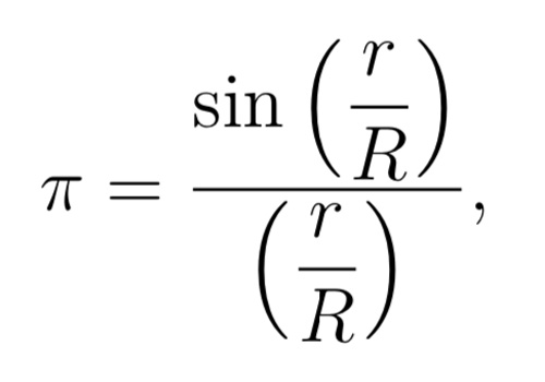
i.e. a smaller value than π, the difference being the more considerable, the greater is the radius of the circle in comparison with the radius R of the “world-sphere.” By means of this relation the spherical beings can determine the radius of their universe (“world”), even when only a relatively small part of their worldsphere is available for their measurements. But if this part is very small indeed, they will no longer be able to demonstrate that they are on a spherical “world” and not on a Euclidean plane, for a small part of a spherical surface differs only slightly from a piece of a plane of the same size.

Thus if the spherical surface beings are living on a planet of which the solar system occupies only a negligibly small part of the spherical universe, they have no means of determining whether they are living in a finite or in an infinite universe, because the “piece of universe” to which they have access is in both cases practically plane, or Euclidean. It follows directly from this discussion, that for our sphere-beings the circumference of a circle first increases with the radius until the “circumference of the universe” is reached, and that it thenceforward gradually decreases to zero for still further increasing values of the radius. During this process the area of the circle continues to increase more and more, until finally it becomes equal to the total area of the whole “world-sphere.”

Perhaps the reader will wonder why we have placed our “beings” on a sphere rather than on another closed surface. But this choice has its justification in the fact that, of all closed surfaces, the sphere is unique in possessing the property that all points on it are equivalent. I admit that the ratio of the circumference c of a circle to its radius r depends on r, but for a given value of r it is the same for all points of the “worldsphere”; in other words, the “world-sphere” is a “surface of constant curvature.”

To this two-dimensional sphere-universe there is a three-dimensional analogy, namely, the three-dimensional spherical space which was discovered by Riemann. its points are likewise all equivalent. It possesses a finite volume, which is determined by its “radius” (2π²R³). Is it possible to imagine a spherical space? To imagine a space means nothing else than that we imagine an epitome of our “space” experience, i.e. of experience that we can have in the movement of “rigid” bodies. In this sense we can imagine a spherical space.

Suppose we draw lines or stretch strings in all directions from a point, and mark off from each of these the distance r with a measuring-rod. All the free end-points of these lengths lie on a spherical surface. We can specially measure up the area (F) of this surface by means of a square made up of measuring-rods. If the universe is Euclidean, then F = 4πr²; if it is spherical, then F is always less than 4πr². With increasing values of r, F increases from zero up to a maximum value which is determined by the “world-radius,” but for still further increasing values of r, the area gradually diminishes to zero. At first, the straight lines which radiate from the starting point diverge farther and farther from one another, but later they approach each other, and finally they run together again at a “counter-point” to the starting point. Under such conditions they have traversed the whole spherical space. It is easily seen that the three-dimensional spherical space is quite analogous to the two-dimensional spherical surface. It is finite (i.e. of finite volume), and has no bounds.

It may be mentioned that there is yet another kind of curved space: “elliptical space.” It can be regarded as a curved space in which the two “counter-points” are identical (indistinguishable from each other). An elliptical universe can thus be considered to some extent as a curved universe possessing central symmetry.

It follows from what has been said, that closed spaces without limits are conceivable. From amongst these, the spherical space (and the elliptical) excels in its simplicity, since all points on it are equivalent. As a result of this discussion, a most interesting question arises for astronomers and physicists, and that is whether the universe in which we live is infinite, or whether it is finite in the manner of the spherical universe. Our experience is far from being sufficient to enable us to answer this question. But the general theory of relativity permits of our answering it with a moderate degree of certainty, and in this connection the difficulty mentioned in Section XXX finds its solution.

APPENDICES

APPENDIX I SIMPLE DERIVATION OF THE LORENTZ TRANSFORMATION (SUPPLEMENTARY TO SECTION XI)

For the relative orientation of the co-ordinate systems indicated in Fig. 2, the x-axes of both systems permanently coincide. In the present case we can divide the problem into parts by considering first only events which are localised on the x-axis. Any such event is represented with respect to the co-ordinate system K by the abscissa x and the time t, and with respect to the system K′ by the abscissa x′ and the time t′. We require to find x′ and t′ when x and t are given.

A light-signal, which is proceeding along the positive axis of x, is transmitted according to the equation

x = ct

or

x – ct = 0 . . . . . (1).

Since the same light-signal has to be transmitted relative to K′ with the velocity c, the propagation relative to the system K′ will be represented by the analogous formula

x′ – ct′ = 0 . . . . . (2)

Those space-time points (events) which satisfy (1) must also satisfy (2). Obviously this will be the case when the relation

(x′ – ct′) = λ(x – ct) . . . (3).

is fulfilled in general, where λ indicates a constant; for, according to (3), the disappearance of (x – ct) involves the disappearance of (x′ – ct′).

If we apply quite similar considerations to light rays which are being transmitted along the negative x-axis, we obtain the condition

(x′ + ct′) = (x + ct) . . . (4).

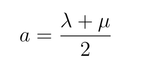
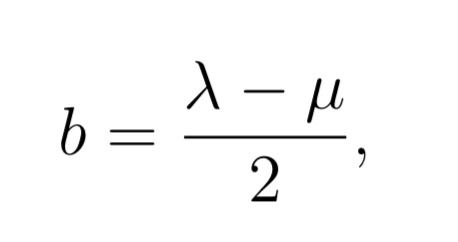
By adding (or subtracting) equations (3) and (4), and introducing for convenience the constants a and b in place of the constants λ and μ where

and

we obtain the equations

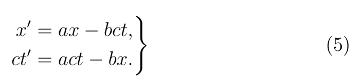
We should thus have the solution of our problem, if the constants a and b were known. These result from the following discussion.

For the origin of K′ we have permanently x′ = 0, and hence according to the first of the equations (5)

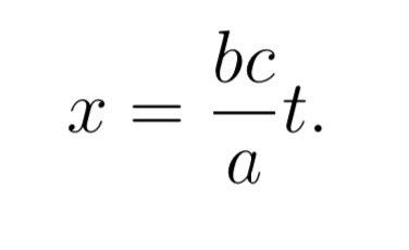
If we call v the velocity with which the origin of K′ is moving relative to K, we then have

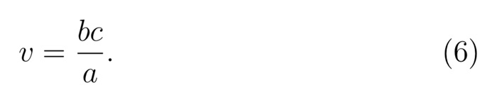
The same value v can be obtained from equations (5), if we calculate the velocity of another point of K′ relative to K, or the velocity (directed towards the negative x-axis) of a point of K with respect to K′. In short, we can designate v as the relative velocity of the two systems.

Furthermore, the principle of relativity teaches us that, as judged from K, the length of a unit measuring-rod which is at rest with reference to K′ must be exactly the same as the length, as judged from K′, of a unit measuring-rod which is at rest relative to K. In order to see how the points of the x′-axis appear as viewed from K, we only require to take a “snapshot” of K′ from K; this means that we have to insert a particular value of t (time of K), e.g. t = 0. For this value of t we then obtain from the first of the equations (5)

x′ = ax

Two points of the x′-axis which are separated by the distance Δx′ = 1 when measured in the K′ system are thus separated in our instantaneous photograph by the distance

But if the snapshot be taken from K′(t′ = 0), and if we eliminate t from the equations (5), taking into account the expression (6), we obtain

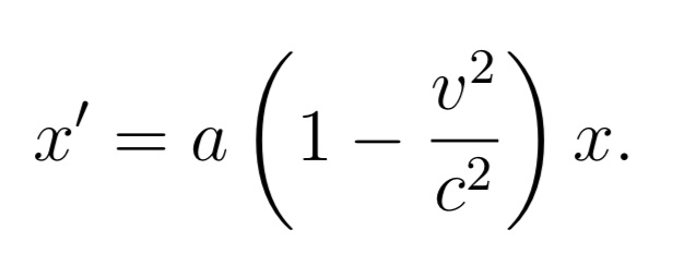
From this we conclude that two points on the x-axis separated by the distance 1 (relative to K) will be represented on our snapshot by the distance

But from what has been said, the two snapshots must be identical; hence Δx in (7) must be equal to Δx′ in (7a), so that we obtain

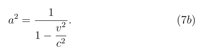
The equations (6) and (7b) determine the constants a and b. By inserting the values of these constants in (5), we obtain the first and the fourth of the equations given in Section XI.

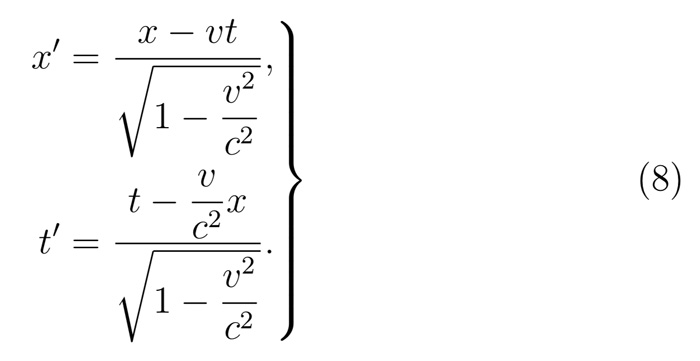
Thus we have obtained the Lorentz transformation for events on the x-axis. It satisfies the condition

x′² – c²t′² = x² – c²t² . . . . . . (8a).

The extension of this result, to include events which take place outside the x-axis, is obtained by retaining equations (8) and supplementing them by the relations

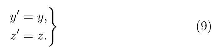
In this way we satisfy the postulate of the constancy of the velocity of light in vacuo for rays of light of arbitrary direction, both for the system K and for the system K′. This may be shown in the following manner.

We suppose a light-signal sent out from the origin of K at the time t = 0. It will be propagated according to the equation

or, if we square this equation, according to the equation

x² + y² + z² – c²t² = 0 . . . . . (10).

It is required by the law of propagation of light, in conjunction with the postulate of relativity, that the transmission of the signal in question should take place—as judged from K′—in accordance with the corresponding formula

r′ = ct′

or,

x′² + y′² + z′² – c²t′² = 0 . . . . . . (10a).

In order that equation (10a) may be a consequence of equation (10), we must have

x′² + y′² + z′² – c²t′² = σ (x² + y² + z² – c²t²) (11).

Since equation (8a) must hold for points on the x-axis, we thus have σ = 1. It is easily seen that the Lorentz transformation really satisfies equation (11) for σ = 1; for (11) is a consequence of (8a) and (9), and hence also of (8) and (9). We have thus derived the Lorentz transformation.

The Lorentz transformation represented by (8) and (9) still requires to be generalised. Obviously it is immaterial whether the axes of K′ be chosen so that they are spatially parallel to those of K. It is also not essential that the velocity of translation of K′ with respect to K should be in the direction of the x-axis. A simple consideration shows that we are able to construct the Lorentz transformation in this general sense from two kinds of transformations, viz. from Lorentz transformations in the special sense and from purely spatial transformations. which corresponds to the replacement of the rectangular co-ordinate system by a new system with its axes pointing in other directions.

Mathematically, we can characterise the generalised Lorentz transformation thus:

It expresses x′, y′, x′, t′, in terms of linear homogeneous functions of x, y, x, t, of such a kind that the relation

x′² + y′² + z′² – c²t′² = x² + y² + z² – c²t² (11a).

is satisficd identically. That is to say: If we substitute their expressions in x, y, x, t, in place of x′, y′, x′, t′, on the left-hand side, then the left-hand side of (11a) agrees with the right-hand side.

APPENDIX II MINKOWSKI’S FOUR-DIMENSIONAL SPACE (“WORLD”) (SUPPLEMENTARY TO SECTION XVII)

We can characterise the Lorentz transformation still more simply if we introduce the imaginary

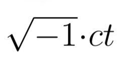
in place of t, as time-variable. If, in accordance with this, we insert

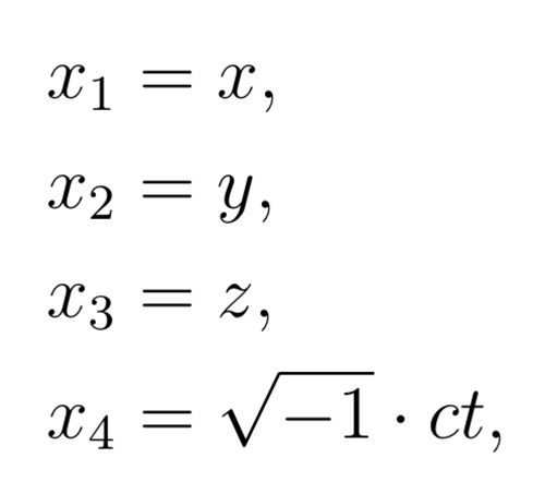
and similarly for the accented system K′, then the condition which is identically satisfied by the transformation can be expressed thus:

x₁′² + x₂′² + x₃′² + x₄′² = x₁² + x₂² + x₃² + x₄² (12).

That is, by the afore-mentioned choice of “coordinates,” (11a) [see the end of Appendix II] is transformed into this equation.

We see from (12) that the imaginary time co-ordinate x₄, enters into the condition of transformation in exactly the same way as the space co-ordinates x₁, x₂, x₃. It is due to this fact that, according to the theory of relativity, the “time” x₄, enters into natural laws in the same form as the space co ordinates x₁, x₂, x₃.

A four-dimensional continuum described by the “co-ordinates” x₁, x₂, x₃, x₄, was called “world” by Minkowski, who also termed a point-event a “world-point.” From a “happening” in three-dimensional space, physics becomes, as it were, an “existence” in the four-dimensional “world.”

This four-dimensional “world” bears a close similarity to the three-dimensional “space” of (Euclidean) analytical geometry. If we introduce into the latter a new Cartesian co-ordinate system (x′₁, x′₂, x′₃) with the same origin, then x′₁, x′₂, x′₃, are linear homogeneous functions of x₁, x₂, x₃ which identically satisfy the equation

x₁′² + x₂′² + x₃′² = x₁² + x₂² + x₃²

The analogy with (12) is a complete one. We can regard Minkowski’s “world” in a formal manner as a four-dimensional Euclidean space (with an imaginary time coordinate); the Lorentz transformation corresponds to a “rotation” of the co-ordinate system in the four-dimensional “world.”

APPENDIX IV THE STRUCTURE OF SPACE ACCORDING TO THE GENERAL THEORY OF RELATIVITY (SUPPLEMENTARY TO SECTION XXXII)

Since the publication of the first edition of this little book, our knowledge about the structure of space in the large (“cosmological problem”) has had an important development, which ought to be mentioned even in a popular presentation of the subject.

My original considerations on the subject were based on two hypotheses:

(1) There exists an average density of matter in the whole of space which is everywhere the same and different from zero.

(2) The magnitude (“radius”) of space is independent of time.

Both these hypotheses proved to be consistent, according to the general theory of relativity, but only after a hypothetical term was added to the field equations, a term which was not required by the theory as such nor did it seem natural from a theoretical point of view (“cosmological term of the field equations”).

Hypothesis (2) appeared unavoidable to me at the time, since I thought that one would get into bottomless speculations if one departed from it.

However, already in the ’twenties, the Russian mathematician Friedman showed that a different hypothesis was natural from a purely theoretical point of view. He realized that it was possible to preserve hypothesis (1) without introducing the less natural cosmological term into the field equations of gravitation, if one was ready to drop hypothesis (2). Namely, the original field equations admit a solution in which the “world radius” depends on time (expanding space). In that sense one can say, according to Friedman, that the theory demands an expansion of space.

A few years later Hubble showed, by a special investigation of the extra-galactic nebulae (“milky ways”), that the spectral lines emitted showed a red shift which increased regularly with the distance of the nebulae. This can be interpreted in regard to our present knowledge only in the sense of Doppler’s principle, as an expansive motion of the system of stars in the large—as required, according to Friedman, by the field equations of gravitation. Hubble’s discovery can, therefore, be considered to some extent as a confirmation of the theory.

There does arise, however, a strange difficulty. The interpretation of the galactic line-shift discovered by Hubble as an expansion (which can hardly be doubted from a theoretical point of view), leads to an origin of this expansion which lies “only” about 10⁹ years ago, while physical astronomy makes it appear likely that the development of individual stars and systems of stars takes considerably longer. It is in no way known how this incongruity is to be overcome.

I further want to remark that the theory of expanding space, together with the empirical data of astronomy, permit no decision to be reached about the finite or infinite character of (three-dimensional) space, while the original “static” hypothesis of space yielded the closure (finiteness) of space.

K = co-ordinate system

x, y = two-dimensional co-ordinates

x, y, z = three-dimensional co-ordinates

x, y, z, t = four-dimensional co-ordinates

t = time

I = distance

v = velocity

F = force

G = gravitational field