Volume 16 — THE GEOMETRY OF THE TRANSLATED NORMAL CURVE.
Reading edition
Carl J. West, Ph. D.
Introduction. In curve tracing the graphic representation is constructed from the equation. Due largely to the requirements of statistics the converse, namely, to find the equation of the curve when the distribution of points is given, has become of interest. This problem is very different from the exercises of analytical geometry in which a given law of distribution of points is to be translated into algebraic language. For the presence in the statistical data of accidental irregularities makes it undesirable as well as practically impossible to obtain a curve passing through the points. Instead, a curve is “fitted” to the points, that is, a curve is passed among the points in accordance with some generally accepted principal such as that of least squares or the agreement of moments.
Aside from the straight line and the parabolas, the curves proposed by Pearson[6] have found acceptance. In order to derive curves which can be fitted to widely varying distributions of points, Professor F. Y. Edgeworth[7] has proposed to modify, to translate, the normal probability curve with unit standard deviation.
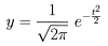
In this article we shall discuss the geometry of the curves which Edgeworth obtains by this transformation and derive a method for an approximate solution of the two equations, one of the fourth and the other of the sixth degree, which arise in the fitting of a curve of this class.
In order that the final curve may be written in terms of the co-ordinates x and y the equation of the base or generating normal probability curve is written:
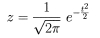
where t denotes abscissas and z ordinates.
Let the abscissas of the transformed curve be functions of the corresponding abscissas of the base curve. Then it may be assumed that x can be developed in powers of t, and hence we may write on omitting fourth and higher powers,
x = a(t + κt2 + λt3),
where a, κ and λ are constants to be determined in “fitting” the curve.
Since x denotes the value of a measurement and y the frequency of x, that is, the number of individuals possessing that value of x, the magnitude of an element of area denotes the number of individuals between two values of x. Obviously, therefore, if the transformation is to be of concrete value the magnitude of an element of area must not be altered, though of course the shape will be changed. Hence
y dx = z dt,
and
y = z dt/dx
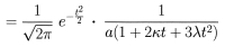
The formulas of transformation are thus:
x = a(t + κt2 + λt3),

Maximum and Minimum Points. Since only curves with one maximum point or mode are practically useful it is desirable to determine what values of the constants a, κ and λ give unimodal curves.
We have
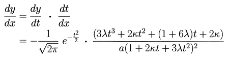
From the vanishing of the numerator of dy/dx there must result either one or three real modes for each pair of values for λ and κ, that is, for each translated curve. To determine what values of λ and κ give uni-modal curves and what tri-modal it is convenient to consider the plane of λ and κ.
The discriminant of the equation
3λt3 + 2κt2 + (1 + 6λ)t + 2κ = 0
is
16κ4 - κ2(1 + 66λ + 117λ2) + 3λ(1 + 6λ)3 = 0
This fourth degree curve crosses the horizontal or λ-axis at λ = 0 and at λ = -⅙ and when λ = 0 its equation reduces to 16κ^4 - κ^2 = 0 or κ = ±0, κ = ±¼. There is thus contact with the vertical or κ-axis at the origin and that axis is crossed at the points (0, ±¼). At the point (λ = -⅙, κ = 0) there is a cusp with the λ-axis for tangent. The other two intersections with the line λ = -⅙ are imaginary, indicating the presence of two branches to the curve.
The discriminant of the denominator of dy/dx is the parabola (in λ and κ),
κ2 - 3λ = 0
The evident close geometrical connection between the two discriminants suggests arranging the discriminant of the cubic curve in the following form:
(κ2 - 3λ) (16κ2 - 117λ2 - 18λ - 1) - 27λ3(1 - 24λ) = 0
From the equation in this, the well known uv + kws = 0 form, numerous elementary geometrical facts can be derived. The relations to the hyperbola, 16κ2 - 117λ2 - 18λ - 1 = 0, and to the parabola, κ2 - 3λ = 0, premit of the ready plotting of the curve with sufficient accuracy. The general shape of the curve is shown in Figure 1.
It is to be noted that one branch of the curve is within the parabola, almost coinciding with it, while the other crosses it at λ = 1/24. From the original form of this equation it appears that the two branches of this discriminant meet just inside the parabola in the end points with approximate co-ordinates (0.043, ±0.360). The geometry of the cusp and end-points on the discriminant curve is suggestive of interesting development in detail.
Values of λ and κ for points on the discriminant give curves with two modes coinciding. All points on one side of the discriminant have three real and distinct modes, and all on the other have one real and two imaginary modes. To determine on which side the points giving three real modes lie we examine a point inside the discriminant. When κ = 0 the modal equation becomes
3λt3 + (1 + 6λ)t = 0.
Hence the roots are
t = 0 and
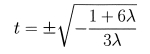
The quantity under the radical is positive for values of λ between 0 and-⅙. Therefore, all points within the discriminant curve yield tri-modal curves and all without uni-modal curves.
The plane of λ and κ
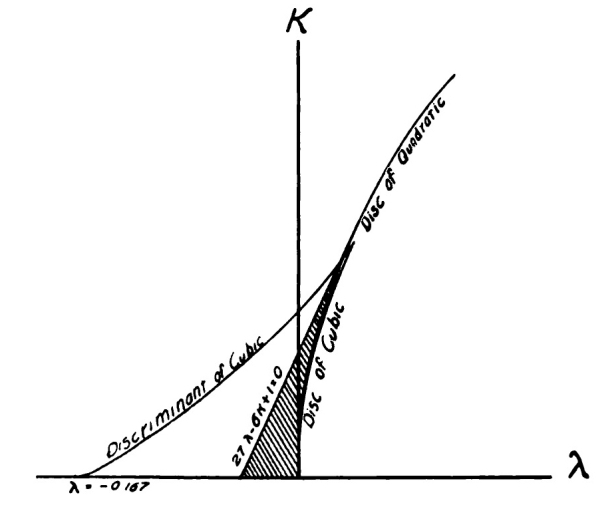
Fig. I
(The horizontal scale is twice the vertical scale)
The infinite values of dy/dx arise from zero values of the quadratic, 1 + 2κt + 3λt2. The greatest possible number of modes for any one curve is therefore five, three from the cubic and two from the quadratic. Since for infinite values of dy/dx the corresponding ordinates are infinite, it is advisable to study the location of the infinite points of the curve, rather to the neglect of the idea of maximum values at such points.
Infinite Ordinates. The infinite points on a curve are given by the values of t satisfying the equation
3λt2 + 2κt + 1 = 0.
Except under certain limited conditions to be determined later a curve with infinite ordinates can not be of great statistical value.
The parabola, κ2-3λ = 0, obtained by equating the discriminant of this quadratic to zero separates the points on the (λ, κ) plane which correspond to curves of no infinite points from those corresponding to curves of two infinite points.
Types of Curves
Therefore, all pairs of values of λ and κ within the parabola, with the exception of the very narrow region also within the first discriminant curve, give uni-modal curves without infinite ordinates.
Types of Curves. Without entering into detailed proofs we will now investigate the general shape of the curves corresponding to values of λ and κ in each of the distinct regions of the plane of λ and κ.
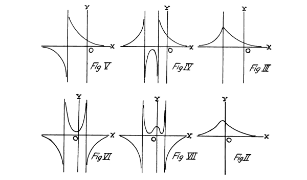
In the region beneath the parabola and to the right from the shaded area of Fig. I the curve is essentially of the shape shown in Fig. II. This type includes the most common skew curves and hence is of great importance in statistics.
As the point (λ, κ) moves from the λ-axis the crest rises until the parabola is reached when the infinite ordinates appear as two coincident lines, shown in Fig. III.
After the parabola is passed, the infinite ordinates separate and the curve apparently separates into three branches as in Fig. IV.
In crossing the κ-axis to the left one asymptote moves off to infinity giving a curve of the type shown in Fig. V.
Then the asymptote reappears giving a curve of the type shown in Fig. VI.
This general shape is preserved as the point moves toward the λ-axis and when the point reaches the discriminant curve the middle branch is flattened at the minimum point.
For points within the discriminant curve two minimum points appear and the central branch now shows a maximum with a minimum point on either side as in Fig. VII.
The Tri-modal Curves. The curves corresponding to values of (λ, κ) within the discriminant, because of the requirement that an element of area under the translated curve must always be equivalent to the corresponding element under the base or generating curve, can be of statistical value only under the following conditions.
The area between the two ordinates corresponding to t = ±3 is 0.99998 of the total area under the curve, so that when neither of the minimum points corresponds to points closer than three units to the origin of the base curve the curve may be practically valuable. A moment’s consideration will show that the abscissas of the two minimum points must be practically the same as that of the corresponding infinite ordinates. The roots of the quadratic
3λt2 + 2κt + 1 = 0
are numerically greater than 3 for all pairs of values of (λ, κ) lying above the line
27λ - 6κ + 1 = 0
As statistically promising within the discriminant of the cubic we then have the shaded area of the (λ, κ) plane.
The Origin. The generating curve is the symmetrical normal probability curve with origin at its center. Since x = 0 when t = 0, the origin of the translated curve coincides with that of the base or generating curve. The translated curve may not be symmetrical so that the mean ordinate may not coincide with the modal ordinate. Because of the relation between corresponding areas the ordinate at the origin must continue to divide the area under the curve into equal parts, that is, the origin and median always coincide.
Determination of the Constants. Since the exact position of the median can not ordinarily be determined by inspection or direct computation there are in reality four constants to be determined: the distance between the median and the mean, a, κ and λ.
In determining the constants it is usual to compute the value of the first four moments. The third and fourth moments are extensions of the idea of the well known formulas for the first and second moments. Denoting the moments about the median by μ, we have
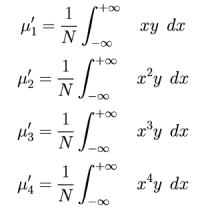
where N is the total area under the curve.
The values of the μ’s are computed from the data[8] and equated to the corresponding integrals which of course involve the four constants. In this way four equations are obtained from which the values of the constants may be determined. Since it is our present object to discuss the solution only of these equations, merely the principal results will be given.
The general form for the moments about the median of the area under the translated curve is
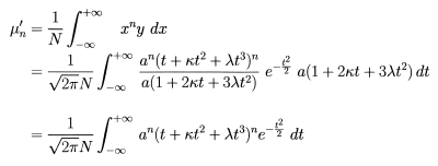
On applying the two well known formulas:
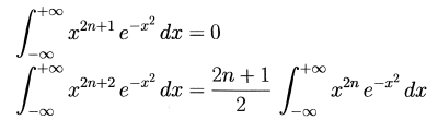
the determination of μ1´, μ2´, μ3´ and μ4´ is reduced to a matter of algebraic detail. Then on transferring to the arithmetic mean as origin the values of μ2, μ3, and μ4 can be determined in terms of a, κ and λ. It is most convenient however, to make use of the quantities β1 = μ32 ⁄ μ23 and β2 = μ4 ⁄ μ22 or rather β = β1 ⁄ 8 and ϵ = (β2 - 3) ⁄ 12 and express the constants in terms of these quantities. It is to be noted that both ϵ and β are zero for a normal distribution, that is, for λ = κ = 0.
Omitting the detailed reduction[9] which is straightforward and direct, we have
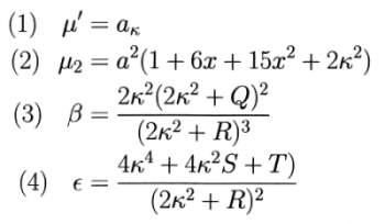
Obviously no algebraic solution can be obtained from equations (3) and (4) for κ and λ in terms of the computed values β and ϵ, and hence a resort to tables is necessary. The values of β and ϵ for values of κ from 0 to 0.0335 and of λ from -0.040 to +0.100 have been computed.[10] The process of determining the constants of the translated normal curve consists first in computing β and ϵ from the given data, and then in entering the table and interpolating for the corresponding values of κ and λ.[11] On substituting these values in (2) the value of a can be found and thence on multiplying a by κ the position of the median of the distribution is obtained.
The sign of κ is determined by the sign of the third moment about the mean μ3, that is, by the direction of the skewness or asymmetry. For positive skewness the mean must lie to the right of the median and hence μ1´, the first moment about the mean, must be positive which necessitates a positive sign for κ. Therefore, the sign of κ is the same as that of the skewness.
To fit a curve to the given data, after the constants have been determined it is necessary to find, by solving a cubic equation for each value, the values of t corresponding to the x’s of the respective classes. The cubic is
aλt3 + aκt2 + at - x = 0.
Any of the various methods of approximating to the solution of a cubic may be used in solving these equations.
The area of each class can now be obtained by computing the corresponding areas under the standard normal curve from a table of the probability integral.
The Method of Interpolation. The actual fitting of the curve can now be readily accomplished.[12] The distinctively geometrical operation is the interpolation for the values of λ and κ for a given pair of values of β and ϵ.
Within the limits of the table[13] the curves resulting from the assignment of a constant value to β are practically straight lines, β = 0 is the λ-axis; β = 1 is a line parallel to the λ-axis. Hence we may safely assume that the variation from one column to the next and from one line to the next is linear for values of β. That is, ordinary first difference interpolation methods are applicable.
As regards the system of ϵ curves we have for instance ϵ = .128 at (λ = .050, κ = 0); again, at approximately (.045, .060) and (.40, .085). We are therefore warranted in assuming the applicability of first difference methods to interpolation between the ϵ curves.
As an illustration let us find the values of λ and κ for ϵ = 0.112 and β = 0.044. On inspection of the table it is seen that λ lies between 0.30 and .035 and κ between .090 and .095. When κ = .090, λ = .033 for ϵ = .112. When κ = .095, λ = .031 for ϵ = .112. For β = .042 and κ = .090, λ = .033 and for β = .046 and κ = .095, λ = .031, ϵ = .112 in each case. Hence, to first differences, λ = .032 and κ = .093 for ϵ = .112 and β = .044. For interpolation in parts of the table showing more rapid variations appropriate methods will suggest themselves.
Taken geometrically the table represents two distinct systems of curves, with each curve of one system intersecting all the curves of the other system. Therefore, a pair of values for λ and κ can always be found for values of ϵ and β within the range of the table.
Department of Mathematics, Ohio State University.
TABLE OF ϵ AND β.
(ϵ is the first and β the second number of each pair.)
λ
κ -040 -035 -030 -025 -020 -015 -010 -005 000
000 -061 -056 -050 -043 -035 -027 -019 -010 000
000 000 000 000 000 000 000 000 000
005 -055 -049 -042 -035 -027 -019 -010 000
000 000 000 000 000 000 000 000
010 -055 -049 -042 -035 -027 -018 -010 000
000 000 000 000 000 000 000 001
015 -049 -042 -035 -027 -018 -009 001
001 001 001 001 001 001 001
020 -048 -041 -034 -026 -017 -008 002
001 002 002 002 002 002 002
025 -047 -040 -033 -025 -016 -007 003
002 002 002 003 003 003 003
030 -046 -039 -032 -024 -015 -006 004
003 003 004 004 004 004 004
035 -045 -038 -031 -023 -014 -005 005
004 005 005 005 005 005 006
040 -037 -030 -022 -013 -004 006
006 006 007 007 007 007
045 -036 -028 -020 -011 -002 008
008 008 008 009 009 009
050 -034 -026 -018 -009 -000 010
009 010 010 011 011 011
055 -032 -024 -016 -007 002 012
011 012 012 013 013 013
060 -022 -014 -005 004 014
014 015 015 016 016
065 -020 -012 -003 006 017
016 017 018 018 019
070 -018 -009 000 009 019
019 020 020 021 022
075 -015 -007 002 012 022
022 023 023 024 025
080 -013 -004 005 015 025
025 026 026 027 028
085 -001 008 018 028
029 030 031 032
090 002 011 021 032
032 033 034 036
095 005 015 025 035
036 037 038 039
100 009 018 028 039
039 041 042 044
(ϵ is the first and β the second number of each pair.)
λ
κ 005 010 015 020 025 030 035 040 045 050
000 010 021 033 045 057 071 084 098 113 128
000 000 000 000 000 000 000 000 000 000
005 010 021 033 045 057 071 084 098 113 128
000 000 000 000 000 000 000 000 000 000
010 011 022 033 045 058 071 085 099 113 128
001 001 001 001 001 001 001 001 001 001
015 011 022 034 046 058 071 085 099 114 129
001 001 001 001 001 001 001 001 001 001
020 012 023 034 046 059 072 086 100 115 130
002 002 002 002 002 002 002 002 002 002
025 013 024 035 047 060 073 087 101 116 131
003 003 003 003 003 003 003 003 003 003
030 014 025 036 049 061 074 088 102 117 132
004 004 004 005 005 005 005 005 005 005
035 015 026 038 050 063 076 089 104 118 133
006 006 006 006 006 006 007 007 007 007
040 017 028 039 052 064 077 091 105 120 135
007 008 008 008 008 008 008 009 009 009
045 019 030 041 053 066 079 093 107 122 137
009 010 010 010 010 011 011 011 011 011
050 021 032 043 055 068 081 095 109 124 139
012 012 012 012 013 013 013 013 014 014
055 023 034 045 057 070 083 097 111 126 141
014 014 015 015 015 016 016 016 016 017
060 025 036 048 060 073 086 100 114 129 144
017 017 017 018 018 019 019 019 019 020
065 028 039 050 062 075 089 102 116 131 146
019 020 020 021 021 022 022 022 023 023
070 030 041 053 065 078 091 105 119 134 149
022 023 024 024 025 026 026 026 026 027
075 033 044 056 068 081 094 108 122 137 152
026 026 027 028 028 029 029 030 030 031
080 036 047 059 071 084 097 111 125 140 155
029 030 031 031 032 033 033 034 034 035
085 039 050 062 075 088 101 115 129 144 159
033 034 034 035 036 037 037 038 039 039
090 043 054 066 079 092 105 119 133 148 163
037 038 039 039 040 041 042 042 043 044
095 046 058 070 083 096 109 123 137 152 167
041 042 043 044 045 046 046 047 048 049
100 050 062 074 087 100 113 127 141 156 171
045 046 047 048 049 050 051 052 053 054
Footnotes: