PART II STATISTICAL TREATMENT OF THE EXPERIMENT

In the discussion and tables which follow:

Q stands for Quotient, which will mean a Subject Age divided by a Chronological Age. R stands for Ratio, which will mean a Subject Age divided by a Mental Age.

AQ means Woody-McCall Arithmetic Age divided by Chronological Age, and AR means this AA divided by Mental Age.

VQ means Thorndike Vocabulary Age divided by Chronological Age, and VR means this VA divided by Mental Age.

RQ means Alpha 2 Reading Age divided by Chronological Age, and RR means this RA divided by Mental Age.

CQ means Kelley-Trabue Completion Age divided by Chronological Age, and CR means this CA divided by Mental Age.

SQ means any Subject Quotient, that is, any Subject Age divided by Chronological Age, and SR means any Subject Ratio, that is, any SA divided by Mental Age.

EQ means the average of all Subject Quotients and AccR, the Accomplishment Ratio, means the average of all Subject Ratios.

All r’s are product-moment correlation coefficients, uncorrected. As the reliabilities (Table 4) are almost what the other coefficients are in June, 1920 (Table 5), it is apparent that the corrected coefficients, when Grade III is excluded, would all be very near unity at that time.

THE QUOTIENTS

In Table 1 are presented all the quotients for all periods of testing, grouped by children. The table, a sample of which is included here,⁠[9] shows clearly how all SQ’s approach IQ as special treatment continues. The grades indicated in this grouping are as of June, 1920. Inasmuch as many double and triple promotions were made in an effort to get maximum product for intelligence invested, no conclusion can here be formed of the grade to which these children belonged at any time except June, 1920. The correspondence between IQ and the SQ’s in June, 1920 is further shown in Table 2. In this table the 48 children who took all tests at all periods are ranked from high to low IQ and their SQ’s are listed opposite. The high correspondence is readily apparent.

TABLE 1⁠[10] Intelligence Quotients for All Periods Grouped by Children

The children are arranged by grade as they were in June, 1920, and alphabetically within the grade. The periods of testing are lettered in their chronological sequence; a is November, 1918, b is June, 1919, c is November, 1919 and d is June, 1920. * = Zero Score

Grade 3

Intelligence Quotient Test Period Arithmetic Quotient Vocabulary Quotient Reading Quotient Completion Quotient

101 a

b

c 64 58 43

d 106 88 93

128 a

b

c 80 102 81

d 152 124 153

116 a

b

c 56 90 * 49

d 94 95 77 89

87 a

b

c 90 40 35 54

d 72 74 61 52

112 a

b

c 90 137 133 112

d 112 113 121 131

TABLE 2⁠[11] Group Taking All Tests at All Periods Arranged in Order of Magnitude of Intelligence Quotients

Intelligence Quotients Arithmetic Quotients Vocabulary Quotients Reading Quotients Completion Quotients

146 111 154 164 150

142 129 135 137 136

141 109 118 107 121

139 124 141 124 134

138 101 112 105 106

138 121 130 110 109

130 107 139 135 136

122 127 130 124 121

122 113 121 117 124

122 112 102 114 129

121 128 125 128 128

120 100 116 102 119

118 117 123 114 125

117 131 111 118 124

117 106 122 112 111

114 105 126 110 114

109 83 113 117 103

107 103 112 95 103

107 94 126 94 123

104 99 117 96 104

104 103 110 94 116

103 108 113 112 106

101 100 114 109 106

100 90 103 92 92

100 109 118 108 113

99 114 104 106 110

99 114 119 117 115

98 102 101 108 104

98 99 106 107 106

97 95 109 107 105

97 108 101 102 105

97 95 104 89 110

96 90 104 91 91

95 84 99 93 100

95 90 107 99 105

95 85 117 114 103

94 106 57 89 108

94 103 103 106 104

92 96 86 94 85

87 83 88 92 87

87 95 96 94 102

84 85 87 93 87

83 106 91 87 104

80 77 91 80 84

80 84 75 79 84

80 89 107 88 86

78 87 90 93 85

60 69 56 71 77

The intercorrelations of the quotients of these 48 cases for all periods may be seen in Table 3 (page 21). The correlations with IQ and the intercorrelations of the SQ’s have increased toward positive unity or rather toward the limits of a correlation with tools of measurement such as we have used. This limit is a function of the reliability of the tests employed. It is customary to use a formula to correct for attenuation in order to find the percentage which the correlation is of the geometric mean of the two reliability coefficients. This is tantamount to saying that any correlation can go no higher than the geometric mean of the reliability coefficients of the tests used. It is better to assume that an r can go as high as the ∜(r₁₁⋅r₂₂) since an r can go as high as the square root of its reliability coefficient. Dr. Truman L. Kelley has shown that the correlation of a test with an infinite number of forms of the same test would be as the square root of its correlation with any one other form.

The reliabilities and limits defining a limit as the fourth root of the multiplied reliability coefficients are in Table 4.

Correction for attenuation is often ridiculously high because the reliability coefficient of one of the measures used is so low. If an element is included in the two tests which are correlated, but not in the other forms of each test used to get reliability, the “corrected coefficient” is corrected for an element which is not chance. Whenever the geometric mean of the reliabilities is less than the obtained r, the corrected r is over 1.00 and hence absurd.⁠[12]

Therefore we use here instead, a comparison to the maximum possibility in a true sense. Since a test correlates with the “true ability” √(r₁₁), ∜(r₁₁⋅r₂₂) is the limit of an r, its optimum with those tools. Although these limits apply, strictly speaking, only to the total correlations, since the reliability correlations are with all the data; we may assume that the same facts hold with regard to the correlations of each of the grades, that is, the reliability is a function of the test not of the data selected.

TABLE 3 Intercorrelation of All Quotients for All Periods of the 48 Children Who Took All Tests

November, 1918

IQ VQ RQ S.D. M

IQ 19.12 105.15

±1.32 ±1.86

VQ .72 20.54 102.52

±.05 ±1.41 ±2.00

RQ .64 .64 19.09 95.90

±.06 ±.06 ±1.31 ±1.86

CQ .63 .71 .77 19.34 99.44

±.06 ±.05 ±.04 ±1.33 ±1.88

June, 1919

IQ VQ RQ S.D. M

IQ 19.12 105.15

±1.32 ±1.86

VQ .73 20.80 113.54

±.05 ±1.43 ±2.02

RQ .65 .58 14.73 101.31

±.06 ±.06 ±1.01 ±1.43

CQ .62 .68 .77 19.76 101.04

±.06 ±.05 +.04 ±1.36 ±1.92

November, 1919

IQ AQ VQ RQ S.D. M

IQ 19.12 105.15

±1.32 ±1.86

AQ .46 14.08 102.90

±.08 ±0.97 ±1.37

VQ .86 .23 17.07 109.17

±.03 ±.09 ±1.18 ±1.66

RQ .65 .56 .71 13.91 101.42

±.06 ±.07 ±.05 ±0.96 ±1.35

CQ .79 .47 .83 .82 17.53 105.21

±.04 ±.08 ±.03 ±.03 ±1.21 ±1.71

June, 1920

IQ AQ VQ RQ S.D. M

IQ 19.12 105.15

±1.32 ±1.86

AQ .73 14.10 101.79

±.05 ±0.97 ±1.37

VQ .81 .60 18.89 108.94

±.03 ±.06 ±1.30 ±1.84

RQ .79 .68 .87 16.43 104.94

±.04 ±.05 ±.02 ±1.13 ±1.60

CQ .84 .77 .78 .84 15.87 108.08

±.03 ±.04 ±.04 ±.03 ±1.09 ±1.54

TABLE 4 Reliability Coefficients

One Form of Each Test Two Forms of Each Test (by Brown’s Formula) One Form with an Infinite Number of Forms Two Forms with an Infinite Number of Forms

r₁₁ r₁₁ √r₁₁ √r₁₁

Intelligence Quotient .888 .942

(by Brown’s Formula)⁠[13]

Arithmetic Quotient .824 .904 .908 .951

Vocabulary Quotient .820 .901 .906 .949

Reading Quotient .866 .928 .931 .963

Completion Quotient .883 .938 .940 .968

Limits of the r’s = ∜(r₁₁ × r₂₂)

Nov. 1918, June and Nov. 1919 June 1920

IQ and AQ .925 .946

IQ and VQ .924 .946

IQ and RQ .936 .953

IQ and CQ .941 .955

The limits of the June, 1920 r’s are naturally somewhat larger than the others since two forms of tests (except the Binet) were used; the unreliability of the quantitative indices is therefore lower and hence the correlation with IQ may be larger.

The correlations in 1920 of another group—the whole school except Grade III—are reproduced in Table 5. Grade III was excluded since here there had as yet been little chance to push the r’s. Partials were obtained with these data (Table 6). Little faith may be placed in the relative sizes of these partials, much because the r_VQ.RQ is here only .73 and, in the data presented in Table 3, it is .87. This is due to the fact that the data in Table 3 cover all periods (2 years) while those in Table 5 cover only one. This difference has comparatively slight influence on our general conclusions; but it makes a huge difference in the correlation of RQ and VQ when IQ is rendered constant, whether the one or the other set of data is used. Moreover, the whole logic of arguing for general factors by reduction of partial correlations from the original r has been called gravely into question in Godfrey H. Thomson’s recent work on this subject: “The Proof or Disproof of the Existence of General Ability.” Thomson shows that partial correlation gives one possible interpretation of the facts, but not an inevitable one. Thus we cannot say that because RQ and IQ and RQ and AQ are highly correlated, correlation of IQ and AQ is dependent upon RQ. We can say, however, that it is likely to be. IQ and AQ may be correlated by reason of inclusion of some element not included at all in RQ. The higher the correlations which we deal with the less we need worry about this, and of course correlations of unity exclude any such consideration.

TABLE 5 Intercorrelation of All Quotients in June, 1920. All Children Exclusive of Grade 3 are Here Represented

The P.E.’s are all less than .05

N = 81

IQ Arithmetic Quotient Vocabulary Quotient Reading Quotient

Arithmetic Quotient .733

Vocabulary Quotient .837 .628

Reading Quotient .758 .694 .734

Completion Quotient .821 .770 .825 .801

I therefore draw no conclusions from the comparative size of these partials, nor do I get partials with any of the other data, and rest the case mainly on the high r’s between IQ and SQ’s in 1920; increase in correspondence of the central tendencies and range of the SQ’s by grade with the central tendency and range of the IQ’s of the same data; small intercorrelation of SR’s and negative correlation of AccR with IQ.

The general lowness of the partials (Table 6) does, however, indicate the great causative relation between IQ and disparity of product. The elements still in here are common elements in the tests and the mistreatment of intelligence.

TABLE 6 Partial Correlations of Quotients Irrespective of Intelligence Quotients

N = 81

Arithmetic Quotient Vocabulary Quotient Reading Quotient

Vocabulary Quotient .04

±.07

Reading Quotient .31 .28

±.07 ±.07

Completion Quotient .43 .44 .47

±.08 ±.06 ±.06

What happened by grade in 1918-1919 is summarized in Table 7. What happened by grade in 1919-1920 is summarized in Table 8. Since there were many changes in personnel from 1918-1919 to 1919-1920, we need expect no continuity from Table 7 to Table 8. For the continuous influence of the two years, see Table 3, which includes 48 children taking all tests at all periods.

TABLE 7 All Correlations, Means, and Standard Deviations by Grade, Showing Progress from November, 1918 to June, 1919

I stands for Intelligence Quotient

V stands for Vocabulary Quotient

R stands for Reading Quotient

C stands for Completion Quotient

GRADE r M S.D.

Nov. June Nov. June Nov. June

III I V .467 .633 I 109.89 113.20 I 12.83 15.49

±.12 ±.07 ±1.98 ±1.91 ±1.40 ±1.35

I R .541 .492 V 96.11 109.90 V 21.21 18.69

±.11 ±.09 ±3.28 ±2.30 ±2.32 ±1.63

I C .641 .386 R 82.26 101.40 R 22.58 15.85

±.09 ±.11 ±3.49 ±1.95 ±2.47 ±1.38

C 86.89 108.40 C 22.76 15.79

±3.52 ±1.94 ±2.49 ±1.37

N = 19 30

IV I V .724 .819 I 105.90 104.82 I 18.08 18.21

±.07 ±.05 ±2.73 ±2.98 ±1.93 ±2.11

I R .665 .845 V 97.20 108.53 V 17.26 24.92

±.08 ±.05 ±2.60 ±4.08 ±1.84 ±2.88

I C .596 .717 R 91.06 107.82 R 27.85 10.35

±.10 ±.08 ±4.20 ±1.69 ±2.97 ±1.20

C 101.45 108.12 C 21.53 17.75

±3.25 ±2.90 ±2.30 ±2.05

N = 20 17

V I V .887 .822 I 101.64 99.42 I 24.76 17.63

±.04 ±.05 ±3.56 ±2.73 ±2.52 ±1.93

I R .799 .832 V 100.59 111.58 V 26.71 19.78

±.05 ±.05 ±3.84 ±3.06 ±2.72 ±2.16

I C .818 .890 R 94.59 101.42 R 22.10 12.56

±.05 ±.03 ±3.18 ±1.94 ±2.25 ±1.37

C 97.00 102.68 C 22.52 17.71

±3.24 ±2.74 ±2.29 ±1.94

N = 22 19

VI I V .793 .772 I 109.90 115.90 I 23.45 24.38

±.08 ±.09 ±5.00 ±5.20 ±3.54 ±3.68

I R .497 .726 V 108.00 126.80 V 30.20 25.25

±.16 ±.10 ±6.44 ±5.39 ±4.55 ±3.81

I C .798 .891 R 103.10 107.20 R 13.77 20.62

±.08 ±.04 ±2.94 ±4.40 ±2.08 ±3.11

C 108.90 117.10 C 15.23 18.81

±3.25 ±4.01 ±2.30 ±2.84

N = 10 10

VII and VIII I V .625 .504 I 99.29 98.92 I 11.11 11.45

±.11 ±.14 ±2.00 ±2.14 ±1.42 ±1.51

I R .622 .709 V 109.43 115.23 V 14.07 17.43

±.11 ±.09 ±2.54 ±2.95 ±1.79 ±2.31

I C .782 .730 R 97.00 98.85 R 12.59 15.77

±.07 ±.09 ±2.27 ±3.26 ±1.61 ±2.09

C 102.43 95.85 C 13.49 17.72

±2.43 ±3.31 ±1.72 ±2.34

N = 14 13

Total I V .685 .680 I 105.07 106.88 I 19.34 18.45

±.04 ±.04 ±1.41 ±1.32 ±1.00 ±0.93

I R .568 .626 V 101.12 112.67 V 22.83 21.58

±.05 ±.04 ±1.67 ±1.54 ±1.18 ±1.09

I C .639 .702 R 92.40 102.91 R 22.65 15.27

±.04 ±.04 ±1.66 ±1.09 ±1.17 ±0.77

C 98.08 106.27 C 21.48 18.19

±1.57 ±1.30 ±1.11 ±0.92

N = 85 89

TABLE 8 All Correlations, Means, and Standard Deviations of Quotients by Grade, Showing Progress from November, 1919 to June, 1920

I stands for Intelligence Quotient

V stands for Vocabulary Quotient

R stands for Reading Quotient

C stands for Completion Quotient

A stands for Arithmetic Quotient

r M S.D.

Nov. June Nov. June Nov. June

III I A .413 .709 I 102.00 105.53 I 9.60 10.89

±.16 ±.08 ±1.87 ±1.68 ±1.32 ±1.19

I V .649 .667 A 82.75 97.84 A 15.88 18.62

±.11 ±.09 ±3.09 ±2.88 ±2.19 ±2.04

I R .651 .609 V 94.00 103.47 V 33.44 27.66

±.11 ±.10 ±6.51 ±4.28 ±4.60 ±3.03

I C .612 .719 R 87.59 93.88 R 32.06 19.02

±.12 ±.07 ±6.24 ±3.21 ±4.41 ±2.27

C 90.17 96.84 C 28.82 25.59

±5.58 ±3.96 ±3.95 ±2.80

N = 12 19

IV I A .426 .725 I 111.48 113.00 I 14.73 15.04

±.10 ±.06 ±1.85 ±1.93 ±1.30 ±1.36

I V .635 .772 A 94.07 111.08 A 12.34 15.02

±.075 ±.05 ±1.55 ±1.99 ±1.09 ±1.40

I R .316 .569 V 109.79 115.61 V 16.97 18.39

±.11 ±.09 ±2.13 ±2.34 ±1.50 ±1.66

I C .594 .837 R 99.31 110.11 R 17.89 14.67

±.08 ±.04 ±3.24 ±1.67 ±1.58 ±1.32

C 108.14 118.14 C 15.51 12.70

±1.94 ±1.62 ±1.37 ±1.15

N = 29 28

V I A .698 .713 I 103.72 98.83 I 19.57 18.84

±.07 ±.07 ±2.69 ±2.65 ±1.91 ±1.87

I V .881 .908 A 87.58 99.71 A 12.43 16.47

±.03 ±.02 ±1.71 ±2.27 ±1.21 ±1.60

I R .773 .891 V 109.00 105.17 V 15.58 19.97

±.06 ±.03 ±2.14 ±2.81 ±1.52 ±1.99

I C .786 .923 R 104.46 103.00 R 16.99 17.07

±.05 ±.02 ±2.34 ±2.40 ±1.65 ±1.70

C 107.00 103.48 C 16.12 14.51

±2.22 ±2.04 ±1.57 ±1.44

N = 24 23

VI I A .533 .805 I 102.43 105.39 I 11.61 13.56

±.13 ±.06 ±2.09 ±2.16 ±1.48 ±1.52

I V .774 .858 A 91.43 104.53 A 11.43 11.31

±.07 ±.04 ±2.06 ±1.75 ±1.46 ±1.24

I R .420 .661 V 106.07 112.94 V 11.93 10.94

±.15 ±.09 ±2.15 ±1.74 ±1.52 ±1.23

I C .739 .620 R 96.64 106.20 R 12.38 11.88

±.08 ±.10 ±2.23 ±1.79 ±1.58 ±1.27

C 100.36 107.61 C 13.95 10.55

±2.51 ±1.68 ±1.78 ±1.19

N = 14 18

VII I A .740 .795 I 107.27 100.58 I 23.29 19.78

±.09 ±.07 ±4.74 ±2.85 ±3.35 ±2.72

I V .867 .718 A 100.00 99.31 A 9.26 11.00

±.05 ±.09 ±1.86 ±2.06 ±1.33 ±1.45

I R .862 .799 V 114.36 108.75 V 19.15 14.42

±.05 ±.07 ±3.89 ±2.81 ±2.75 ±1.98

I C .833 .677 R 101.73 98.58 R 12.28 11.56

±.06 ±.11 ±2.50 ±2.25 ±1.77 ±1.59

C 105.82 101.42 C 17.41 16.02

±3.54 ±3.12 ±2.50 ±2.21

N = 11 12

VIII I A .663 .796 I 104.83 108.79 I 15.46 18.25

±.11 ±.07 ±3.01 ±3.29 ±2.13 ±2.33

I V .828 .750 A 92.92 93.86 A 10.20 9.74

±.06 ±.08 ±1.99 ±1.76 ±1.40 ±1.24

I R .775 .722 V 111.67 117.21 V 16.44 14.02

±.08 ±.08 ±3.20 ±2.53 ±2.26 ±1.79

I C .838 .868 R 100.83 104.38 R 11.52 20.62

±.06 ±.04 ±2.24 ±3.72 ±1.59 ±2.63

C 104.92 109.64 C 18.11 17.41

±3.53 ±3.14 ±2.49 ±2.22

N = 12 14

Total I A .576 .686 I 106.02 105.87 I 16.73 16.87

±.05 ±.03 ±1.12 ±1.07 ±0.79 ±0.75

I V .679 .727 A 91.35 102.01 A 13.22 15.61

±.04 ±.03 ±0.88 ±0.98 ±0.62 ±0.69

I R .529 .609 V 107.95 110.54 V 19.76 19.57

±.05 ±.04 ±1.32 ±1.24 ±0.93 ±0.87

I C .678 .731 R 99.22 103.65 R 18.85 17.12

±.04 ±.03 ±1.26 ±1.08 ±0.89 ±0.76

C 104.06 108.00 C 18.87 18.11

±1.26 ±1.14 ±0.89 ±0.81

N = 102 114

Note—Totals without Grade III are much higher than these (Table 5). Grade III has many children in it who have not been long enough in an academic situation to allow their SQ’s to go as high as they may.

It is proper to note here that not much can be expected from Grades III and VIII and from totals including Grade III, since children in Grade III have not been there long enough to be pushed, and children in Grade VIII have been pushed beyond the limits which the tests used will register. Our logic is one of pushed correlations. If the association of IQ and the SQ’s is what we are attempting to establish, it is necessary to show:

1. That the r comes near unity;

2. That the central tendencies come near coincidence;

3. That the S.D.’s come near coincidence.

The value of the r is obvious; the value of coincidence of means becomes clearer if we think of Σ(IQ-EQ)/n, the average difference of potential rate of progress and actual rate of progress. This average of differences is the same as the difference of the averages, which is more readily calculated. Obviously, if we wish to use an AccR, it is necessary to show more than correspondence when differences in average and spread are equated as they are by the correlation coefficient. Besides, coincidence of M’s, correspondence of S.D.’s is also necessary since a correlation might be positive unity, the M’s might be equal, and still the spread of one measure might be more than the spread of the other. If the spreads are the same and the M’s are the same, and the correlation is positive unity, each x must equal its corresponding y. Then b₁₂ = b₂₁ = 1.00; and the M’s being equal, the deviations are from the same point. Therefore, we will attempt to measure similarity of M’s and S.D.’s as well as r.

It will be observed that both Tables 7 and 8 give evidence of each of these tendencies in all grades. In Table 8 marked progress in arithmetic is apparent. This is due to re-classification in terms of the Woody-McCall test, which was not done in 1918-1919. In 1918-1919 no arithmetic test was given and all re-classification was in terms of reading, being done on the basis of both reading tests. Spelling re-classification was done each year, but the data were not treated in this manner. It can be said that wherever re-classification in terms of intelligence and pedagogical need was undertaken the desired result of pushing the SQ’s up to IQ was hastened. Of all the remedial procedure, such as changing teachers and time allotment and books and method, all of which were employed to some extent, it is my opinion that the re-classification was more important than everything else combined.

It is noticeable that when r’s approach the limit which the unreliability of the test allows them, they drop down again. This is probably due to continued increase of SQ’s over IQ. Of course, for some SQ’s to be greater than IQ out of proportion to the general amount lowers the correlation as much as for some to lag behind. When the SQ’s of the children of lower intelligence reach their IQ they continue above. This, of course, is due to errors in establishment of the age norms. The norms are not limits of pushing, though an attempt was made by correction for truncation to get them as nearly so as possible. It is to be noted, however, that these norms are up the growth curve, that is, reading age of 10 means a score such that the average age of those getting it is 10, not the average score of children whose mental age is 10. The average reading achievement of children all ten years old chronologically is higher than that of a group all mentally ten, since many of the mentally advanced have not been pushed in product. The group used here to establish norms gives more nearly pushed norms than the others would.

The tendency of the low IQ’s to go over unity in their SR’s is apparent in Table 1 and in Table 12 and also in the negative correlation between AccR and IQ.

In both years some second grade children were advanced to Grade III during the year. This accounts for the low r’s in June, 1919, but in 1919-1920 the Grade III correlations are raised and the means raised toward the M_IQ, even though some second grade children were put in this group during the year.

TABLE 9 Summary of Progress in Arithmetic by Increase in r, Decrease in M_IQ-M_AQ and Decrease in Difference of Standard Deviations Irrespective of Direction

GRADE r Average Intelligence Quotient Minus Average Arithmetic Quotient Difference of Standard Deviations Irrespective of Sign (of IQ and Arith. Q)

Nov. June Nov. June Nov. June

III .413 .709 19.25 8.16 6.27 6.63

±.16 ±.08 ±2.87 ±2.05 ±2.04 ±1.45

IV .426 .725 7.41 0.46 2.39 0.47

±.10 ±.06 ±1.84 ±1.50 ±1.29 ±1.02

V .698 .713 16.14 0.54 7.14 2.06

±.07 ±.07 ±1.93 ±1.84 ±1.37 ±1.30

VI 5.33 .805 11.00 3.00 0.19 1.63

±.13 ±.06 ±2.01 ±1.19 ±1.42 ±0.85

VII .740 .795 7.27 0.62 14.03 8.15

±.09 ±.07 ±3.58 ±2.33 ±2.53 ±1.63

VIII .663 .796 11.92 [14]⁠14.93 5.26 [14]⁠8.53

±.11 ±.07 ±2.25 ±2.69 ±1.59 ±1.54

Total .576 .686 14.67 3.72 3.51 1.16

±.05 ±.03 ±0.94 ±0.81 ±0.67 ±0.57

TABLE 10 Summary of Progress in Reading, November, 1918 to June, 1919, by Increase in r, Decrease in M_IQ-M_RQ, and Decrease in Difference of Standard Deviations Irrespective of Sign

GRADE r Average Intelligence Quotient Minus Average Reading Quotient Difference of Standard Deviations Irrespective of Sign (of IQ and RQ)

Nov. June Nov. June Nov. June

III .541 .492 27.63 11.80 9.75 0.36

±.11 ±.09

IV .665 .845 14.84 -3.00 9.77 7.86

±.08 ±.05

V .799 .832 7.05 -2.00 2.66 5.07

±.05 ±.05

VI .497 .726 6.80 8.70 9.68 3.76

±.16 ±.10

VII .622 .709 2.28 0.07 1.48 5.98

3 of VIII ±.11 ±.09

Total .568 .626 12.67 3.97 3.31 3.18

±.05 ±.04

TABLE 11 Summary of Progress in Reading, November, 1919 to June, 1920, by Increase in r, Decrease in M_IQ-M_RQ, and Decrease in Difference of Standard Deviations Irrespective of Sign

GRADE r Average Intelligence Quotient Minus Average Reading Quotient Difference of Standard Deviations Irrespective of Sign (of IQ and RQ)

Nov. June Nov. June Nov. June

III .651 .609 14.41 11.57 22.46 8.62

±.11 ±.10 ±5.22 ±2.55 ±3.69 ±1.81

IV .316 .569 12.17 2.43 3.16 0.76

±.11 ±.09 ±2.41 ±1.78 ±1.70 ±1.26

V .773 .891 -0.74 -4.17 2.58 1.77

±.06 ±.03 ±1.72 ±1.20 ±1.22 ±0.85

VI .420 .661 5.79 0.90 0.77 0.87

±.15 ±.09 ±2.33 ±1.53 ±1.65 ±1.09

VII .862 .799 5.54 0.92 11.00 8.31

±.05 ±.07 ±2.88 ±2.54 ±2.03 ±1.80

VIII .775 .722 4.00 4.43 3.94 2.41

±.08 ±.09 ±1.90 ±2.64 ±1.92 ±1.87

Total .529 .609 6.80 2.86 2.12 0.06

±.05 ±.04 ±1.16 ±0.30 ±0.82 ±0.67

The changes in rates of progress are expressed in summaries by subject matter in Tables 9, 10, and 11. Approach of Arithmetic Quotient to Intelligence Quotient is measured in Table 9 by:

1. Comparison of r in June with r in November.

2. Comparison of M_IQ-M_AQ in June and M_IQ-M_AQ in November.

3. Comparison of S.D.’s of Arithmetic and Intelligence Quotients in June and November.

The P.E.’s of each of these differences were obtained by

P.E._diff² = P.E.₁² + P.E.₂² - 2 r₁₂ P.E.₁ P.E.₂

The only M_IQ-M_SQ in Table 9 which does not show a decrease at least two times as large as the P.E. of either of the elements involved, is the 8th grade; and this is due to the limits of the test used. As mentioned before, the 8th grade did not register its true abilities in June since a perfect, or nearly perfect, score in the test was too easy to obtain. The small arithmetic S.D.’s in Grade 8 and consequent great S.D._IQ-S.D._SQ is due to the same cause.

Tables 10 and 11 present the summary of facts with regard to Thorndike Reading Quotients, the first and second years respectively.

THE RATIOS

The discussion which follows concerns Ratios, not Quotients.

TABLE 12 Intelligence Quotients and Subject Ratios for All Periods Grouped by Child. The Order of Entries is Just as in Table 1

Grade III

Intelligence Quotient Arithmetic Ratio Vocabulary Ratio Reading Ratio Completion Ratio

101 a

b

c 63 57 43

d 105 87 92

128 a

b

c 62 80 63

d 119 97 120

116 a

b

c 48 78 * 42

d 81 82 66 77

87 a

b

c 103 46 40 62

d 83 85 70 60

112 a

b

c 80 122 119 100

d 100 101 108 117

101 a

b

c 84 93 37 55

d 90 110 98 92

90 a

b

c 76 58 72 89

d 68 121 77 102

105 a

b

c 60 43 * 57

d 104 95 83 66

The remainder of this table is filed in Teachers College Library, Columbia University.

TABLE 13

Nov., 1918 June, 1919 Nov., 1919 June, 1920

Means

Arithmetic Ratio 89.02 97.16

±1.05 ±1.07

Vocabulary Ratio 98.96 111.44 106.20 107.61

±1.48 ±1.61 ±0.90 ±0.93

Reading Ratio 96.47 101.96 98.98 100.60

±1.19 ±1.18 ±1.03 ±0.97

Completion Ratio 99.76 101.83 101.67 103.10

±1.11 ±1.23 ±0.93 ±0.85

Standard Deviations

Arithmetic Ratio 12.03 12.53

±0.74 ±0.76

Vocabulary Ratio 15.71 16.58 10.34 10.84

±1.05 ±1.14 ±0.64 ±0.66

Reading Ratio 12.63 12.14 11.82 11.36

±0.84 ±0.84 ±0.73 ±0.69

Completion Ratio 12.34 12.63 10.85 9.90

±0.82 ±0.87 ±0.67 ±0.60

Correlations of Ratios

Arithmetic and Vocabulary .60 .30

±.06 ±.08

Arithmetic and Reading .70 .64

±.04 ±.05

Arithmetic and Completion .48 .61

±.07 ±.05

Vocabulary and Reading .34 .32 .57 .47

±.08 ±.09 ±.06 ±.07

Vocabulary and Completion .45 .36 .53 .54

±.07 ±.08 ±.06 ±.06

Reading and Completion .61 .65 .67 .67

±.06 ±.06 ±.05 ±.05

In Table 12 are presented the Subject Ratios in the same order as the Quotients appear in Table 1.⁠[15] There plainly is a rapid rise of SQ/IQ from period to period, excluding all pupils who did not take all tests and excluding Grade III; which includes all children taking all tests who were in school in June, 1920, and were Grade IV and above in November, 1918. The average AccR is 98.24 in November, 1918, and 102.78 in June, 1920. The average IQ for these children is 105.22. The S.D_{AccR₁₉₁₈} is 11.17; the S.D._{AccR₁₉₂₀} is 9.09; the S.D._IQ is 19.24. It is obvious that the average amount of product per intelligence has increased, that the range of AccR’s has decreased (which means that factors causing disparities, other than intelligence, have been removed), and that the S.D. of the AccR’s is about one half the S.D. of the IQ’s. M’s are about equal so it is not necessary to use coefficients of variability. The variability of children, intelligence aside, is only one half what the variability is otherwise. The correlations when IQ = X, AccR₁₉₁₈ = Y and AccR₁₉₂₀ = S and when AccR = average of Vocabulary, Reading and Completion Ratios, are:⁠[16]

r_X.Y. = -.602

r_X.S. = -.493

r_Y.S. = +.549

The remaining disparity is then due to something which is in negative correlation with intelligence.

The number of cases here is only 48.

The P.E.’s are then as follows:

P.E._M P.E._S.D.

X 1.91 1.35

Y 1.11 0.79

S 0.90 0.64

P.E.r_X.Y. = .06

P.E.r_X.S. = .08

P.E.r_Y.S. = .07

The differences between the M’s and between the S.D.’s of our 1918 and our 1920 AccQ’s; namely, 102.78 - 98.24 = 4.54 and 11.17 - 9.09 = 2.08, have formed a step in the argument. We must have the P.E.’s of these amounts in order to establish the reliability of the quantitative indices we employ:

P.E._diff = √P.E._X² + P.E._Y² - 2 r_XY P.E._X P.E._Y

P.E._{M₂₀-M₁₈} = 0.94

P.E._{S.D.₁₈-S.D.₂₀} = 0.47

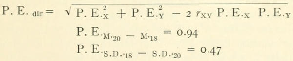
These differences are then reliable. If the same data were accumulated again in the same way with only 48 cases, the chances are even that the 4.54 would be between 3.50 and 5.48 and the 2.08 between 1.61 and 2.55. That there would be positive differences is practically certain, since the difference between the means is over four times as large as its P.E., and the difference between the S.D.’s over four times as large as its P.E.

To make still more certain this observation of positive amount in M of second testing minus M of first testing and in S.D. of first testing minus S.D. of second testing (AccR), which means an increase in central tendency of AccR’s and a decrease in spread of AccR’s under special treatment, we have listed in Table 13 the means and standard deviations of Subject Ratios of each test for each period and the intercorrelations of these Subject Ratios. These do not include exactly the same children in each period but are inclusive of all grades for all periods. They are a measurement of increased efficiency of the school as a whole, rather than of any one group of children; though, of course, the bulk of the children have representation in each of these indices. Too much continuity is not to be expected from June, 1919, to November, 1919, as the children are different. Comparison should always be from November to June.

These tables bear out the fact presented by AccR. It is clear that there is a marked development in the S.R.’s, both by increase of M. and decrease of S.D. The decrease of correlation between S.R.’s is not so marked, but neither is the negative correlation between AccR and IQ much less in June, 1920, than in November, 1918. The association of achievements in terms of intelligence is very probably due to mistreatment, since it is in negative correlation with IQ, as a general inherited ethical factor could not be.

We will note that the Arithmetic Ratios are in as high positive association with the Reading Ratios as the Vocabulary Ratios are with the Reading Ratios. This makes it highly improbable that the intercorrelation of these remnants is due, to any large extent, to common elements in the test or to specific abilities. The common interassociation of all Ratios seems to point to the operation of some common factor other than intelligence as a determinant of disparity in school progress. It would be easy to identify this as the part of Burt’s “General Educational Factor” which is not intelligence—that is, industry, general perseverance and initiative—were it not for the fact that this same influence stands in negative association to intelligence. It is our belief that it is the influence of a maladjusted system of curricula and methods which accounts for these rather high interassociations of achievements, irrespective of intelligence.

SUMMARY

The association of abilities in arithmetic, reading, and completion with intelligence is markedly raised by special treatment. Disparities of educational product are therefore to a great extent due to intelligence. (Tables 2, 3, 5, 7, 8, 9, 10 and 11.)

The remnants (intelligence being rendered constant by division of each SQ by IQ) intercorrelate about .5. If there were specialized inherited abilities, these intercorrelations would not all be positive nor would they be as uniform. (Tables 6 and 13.)

The averages of these remnants, for reading, vocabulary, and completion, correlate -.61 in 1918 and -.49 in 1920 with IQ. These remnants are in negative association to intelligence. If the intercorrelations of these remnants were due to a “General Factor,” this correlation would not be negative.

Therefore intelligence is far and away the most important determinant of individual differences in product.

As part of the relation between tests, irrespective of intelligence, is due to common elements in the tests, this reasoning becomes still more probable.

General factor in education, as distinct from intelligence, has not been separated here from inherited bases of ambition, concentration, and industry. It seems out of our province to conjure up some inherited complex of abilities other than intelligence, specialized inherited abilities, or proclivities and interests tending to thorough prosecution of school work. I have therefore meant this last by the general factor.

McCall has correlations varying continually in size from -.63 to +.98 between various measurements of a group of 6B children.⁠[17] The abilities involved were not pushed as are those considered here. Some of the low correlations are no doubt indications of low association because of the way children are, not the way they might be by heritage; still others, such as handwriting and cancellation (unless bright children do badly in cancellation tests because they are more bored than the others), are correlated low or negatively with intelligence when the correlation is at its maximum. Such results as those of McCall serve as a guide not to argue about other tests by analogy. It is necessary to find which traits and abilities can be pushed to unity in their relation to intelligence and which, like handwriting, are practically unrelated to general mental power.

It is well to know about music tests and such tests as Stenquist’s mechanical ability test when the correlation with intelligence is pushed, before we decide whether the quality measured is a manifestation of specific talent or general intelligence.

Cyril Burt obtained data much like that presented here except that instead of getting rid of the influence of intelligence and finding determinants for the remnants of disparity, he built up a hierarchy of coefficients as they would be if they were due entirely to a common factor and compared these with his obtained r’s. I will present his conclusions with regard to a general factor which are in substantial though not complete agreement with those advanced here.

“Evidence of a Single Common Factor.

“The correlations thus established between the several school subjects may legitimately be attributed to the presence of common factors. Thus, the fact that the test of Arithmetic (Problems) correlates highly with the test of Arithmetic (Rules) is most naturally explained by assuming that the same ability is common to both subjects; similarly, the correlation of Composition with Arithmetic (Problems) may be regarded as evidence of a common factor underlying this second pair; and so with each of the seventy-eight pairs. But is the common factor one and the same in each case? Or have we to recognise a multiplicity of common factors, each limited to small groups of school subjects?

“To answer this question a simple criterion may be devised. It is a matter of simple arithmetic to reconstruct a table of seventy-eight coefficients so calculated that all the correlations are due to one factor and one only, common to all subjects, but shared by each in different degrees. Such a theoretical construction is given in Table XIX. In this table theoretical values have been calculated so as to give the best possible fit to the values actually obtained in the investigation, and printed in Table XVIII. It will be seen that the theoretical coefficients exhibit a very characteristic arrangement. The values diminish progressively from above downwards and from right to left. Such an arrangement is termed a ‘hierarchy.’ Its presence forms a rough and useful criterion of the presence of a single general factor.

“On turning to the values originally obtained (Table XVIII.) it will be seen that they do, to some extent, conform to this criterion. In certain cases, however, the correlations are far too high—for instance, those between Arithmetic (Rules) and Arithmetic (Problems), and again Drawing and both Handwork and Writing (Quality). Now these instances are precisely those where we might anticipate special factors—general arithmetical ability, general manual dexterity—operating over and above the universal factor common to all subjects. These apparent exceptions, therefore, are not inconsistent with the general rule. Since, then, the chief deviations from the hierarchical arrangement occur precisely where, on other grounds, we should expect them to occur, we may accordingly conclude that performances in all the subjects tested appear to be determined in varying degrees by a single common factor.

“Nature of the Common Factor.

“What, then, is this common factor? The most obvious suggestions are that it is either (1) General Educational Ability or (2) General Intelligence. For both these qualities, marks have been allotted by teachers, quite independently of the results of the tests. The correlations of these marks with performances in the tests are given in the last two lines of Table XVIII.

“Upon certain assumptions, the correlation of each test with the Hypothetical Common Factor can readily be deduced from the coefficients originally observed. These estimates are given in the last line but two of the table. They agree more closely with the observed correlations for General Educational Ability, especially if the latter are first corrected for unreliability. (Correlations: Hypothetical General Factor coefficients and General Educational Ability coefficients .86; after correction .84. Hypothetical General Factor coefficients and General Intelligence coefficients .84; after correction .77.) We may, therefore, identify this hypothetical general factor with General Educational Ability, and conclude provisionally that this capacity more or less determines prowess in all school subjects.

“The high agreement of the estimated coefficients with the intelligence correlations suggest that General Intelligence is an important, though not the only factor in General Educational Ability. Other important factors are probably long-distance memory, interest and industry. It is doubtless not a pure intellectual capacity; and, though single, is not simple, but complex.”⁠[18]