Conceptual Design of Self-Organizing Machines

P. A. Kleyn

Northrop Nortronics Systems Support Department Anaheim, California

Self-organization is defined and several examples which motivate this definition are presented. The significance of this definition is explored by comparison with the metrization problem discussed in the companion paper (1) and it is seen that self-organization requires decomposing the space representing the environment. In the absence of a priori knowledge of the environment, the self-organizing machine must resort to a sequence of projections on unit spheres to effect this decomposition. Such a sequence of projections can be provided by repeated use of a nilpotent projection operator (NPO). An analog computer mechanization of one such NPO is discussed and the signal processing behavior of the NPO is presented in detail using the Euclidean geometrical representation of the metrizable topology provided in the companion paper. Self-organizing systems using multiple NPO’s are discussed and current areas of research are identified.

INTRODUCTION

Unlike the companion paper which considers certain questions in depth, this paper presents a survey of the scope of our work in self-organizing systems and is not intended to be profound.

The approach we have followed may be called phenomenological (Figure 1). That is, the desired behavior (self-organization) was defined, represented mathematically, and a mechanism(s) required to yield the postulated behavior was synthesized using mathematical techniques. One advantage of this approach is that it avoids assumptions of uniqueness of the mechanism. Another advantage is that the desired behavior, which is after all the principal objective, is taken as invariant. An obvious disadvantage is the requirement for the aforementioned synthesis technique; fortunately in our case a sufficiently general technique had been developed by the author of the companion paper.

From the foregoing and from the definition of self-organization we employ (see conceptual model), it would appear that our research does not fit comfortably within any of the well publicized approaches to self-organization (2). Philosophically, we lean toward viewpoints expressed by Ashby (3), (4), Hawkins (5), and Mesarovic (6) but with certain reservations. We have avoided the neural net approach partly because it is receiving considerable attention and also because the brain mechanism need not be the unique way to produce the desired behavior.

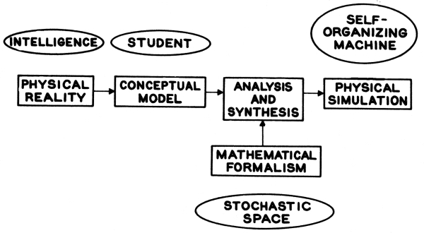
Figure 1—Approach used in Nortronics research on self-organizing systems

Nor have we followed the probability computer or statistical decision theory approach exemplified by Braverman (7) because these usually require some sort of preassigned coordinate system (8). Neither will the reader find much indication of formal logic (9) or heuristic (10) programming. Instead, we view a self-organizing system more as a mirror whose appearance reflects the environment rather than its own intrinsic nature. With this viewpoint, a self-organizing system appears very flexible because it possesses few internal constraints which would tend to distort the reflection of the environment and hinder its ability to adapt.

CONCEPTUAL MODEL

Definition

A system is said to be self-organizing if, after observing the input and output of an unknown phenomenon (transfer relation), the system organizes itself into a simulation of the unknown phenomenon.

Implicit in this definition is the requirement that the self-organizing machine (SOM) not possess a preassigned coordinate system. In fact it is just this ability to acquire that coordinate system implicit in the input-output spaces which define the phenomenon that we designate as self-organization. Thus any a priori information programmed into the SOM by means of, for example, stored or wired programs, constrains the SOM and limits its ability to adapt. We do not mean to suggest that such preprogramming is not useful or desirable; merely that it is inconsistent with the requirement for self-organization. As shown in Figure 2, it is the given portion of the environment which the SOM is to simulate, which via the defining end spaces, furnishes the SOM with all the data it needs to construct the coordinate system intrinsic to those spaces.

The motivation for requiring the ability to simulate as a feature of self-organization stems from the following examples.

Consider the operation of driving an automobile. Figure 3 depicts the relation characterized by a set of inputs; steering, throttle, brakes, transmission, and a set of outputs; the trajectory. Operation of the automobile requires a device (SOM) which for a desired trajectory can furnish those inputs which realize the desired trajectory. In order to provide the proper inputs to the automobile, the SOM must contain a simulation of ⨍⁻¹(x).

Figure 2—Simulation of (a portion of) the environment

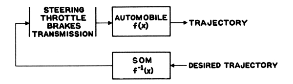
Figure 3—Simulation of a relation

Since ⨍(x) is completely defined in terms of the inputs and the resulting trajectories, exposure to them provide the SOM with all the information necessary to simulate ⨍⁻¹(x). And if the SOM possesses internal processes which cause rearrangement of the input-output relation of the SOM to correspond to ⨍⁻¹(x) in accordance with the observed data, the SOM can operate an automobile. It is this internal change which is implied by the term “self-organizing,” but note that the instructions which specify the desired organization have their source in the environment.

As a second example consider adaptation to the environment. Adapt (from Webster) means: “to change (oneself) so that one’s behavior, attitudes, etc., will conform to new or changed circumstances. Adaptation in biology means a change in structure, function or form that produces better adjustment to the environment.” These statements suggest a simulation because adjustment to the environment implies survival by exposing the organism to the beneficial rather than the inimical effects of the environment. If we represent the environment (or portion thereof) as a relation as shown in Figure 2, we note that the ability to predict what effect a given disturbance will have is due to a simulation of the cause-effect relation which characterizes the environment.

It would be a mistake to infer from these examples that simulation preserves the appearance of the causes and effects which characterize a relation. We clarify this situation by examining a relation and its simulation.

Consider the relation between two mothers and their sons as pictured in Figure 4. Observe that if symbols (points) are substituted for the actual physical objects (mothers and sons), the relation is not altered in any way. This is what we mean by simulation and this is how a SOM simulates. It is not even necessary that the objects, used to display the relation, be defined; i.e., these objects may be primitive. (If this were not so, no mathematical or physical theory could model the environment.) The main prerequisite is sufficient resolution to distinguish the objects from each other.

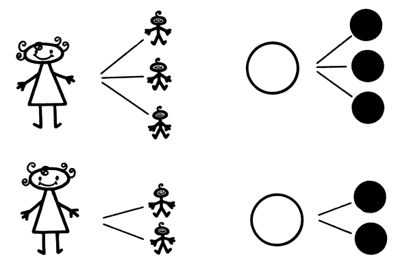
Figure 4—A relation of objects—displayed and simulated

MATHEMATICAL MODEL

The mathematical model must represent both the environment and the SOM and for reasons given in the companion paper each is represented as a metrizable topology. For uniqueness we factor each space into equal parts and represent the environment as the channel

W ⟶ X. (Ref. 10a)

Consider now the SOM to be represented by the cascaded channels

X ⟶ Y ⟶ Z

where X ⟶ Y is a variable which represents the reorganization of the SOM existing input-output relation represented by Y ⟶ Z.

The solution of the three channels-in-cascade problem

W ⟶ X ⟶ Y ⟶ Z,

where p(W) (11), p(X), p(X|W), p(Y), p(Z), p(Z|Y) are fixed, yields that middle channel p₀(Y|X), from a set of permissible middle channels {p(Y|X)}, which maximizes R(Z,W).

Then the resulting middle channel describes that reorganization of the SOM which yields the optimum simulation of W ⟶ X by the SOM, within the constraints upon Ch(Z,Y).

The solution (the middle channel) depends of course on the particular end channels. Obviously the algorithm which is used to find the solution does not. It follows that if some physical process were constrained to carrying out the steps specified by the algorithm, said process would be capable of simulation and would exhibit self-organization.

Although the formal solution to the three-channels-in-cascade problem is not complete, the solution is sufficiently well characterized to permit proceeding with a mechanization of the algorithm. A considerable portion of the solution is concerned with the decomposition and metrization of channels and it is upon this feature that we now focus attention.

As suggested in the companion paper, if the dimensionality of the spaces is greater than one, the SOM has only one method available (12). Consider the decomposition of a space without, for the moment, making the distinction between input and output.

Figure 5 depicts objects represented by a (perhaps multidimensional) “cloud” of points. In the absence of a preassigned coordinate system, the SOM computes the center of gravity of the cloud (which can be done in any coordinate system) and describes the points in terms of the distance from this center of gravity; or, which is the same, as concentric spheres with origin at the center of gravity.

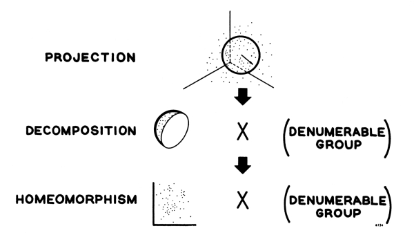
Figure 5—Nilpotent decomposition of a three-dimensional space

The direction of particular point cannot be specified for there is no reference radius vector. Since the SOM wants to end up with a cartesian coordinate system, it must transform the sphere (a two-dimensional surface) into a plane (a two-dimensional surface). Unfortunately, a sphere is not homeomorphic to a plane; thus the SOM has to decompose the sphere into a cartesian product of a hemisphere (12a) and a denumerable group. The SOM then can transform the hemisphere into a plane. The points projected onto the plane constitute a space of the same character as the one with which the SOM started. Thus, it can repeat all operations on the plane (a space of one less dimension) by finding the center of gravity and the circle upon which the desired point is situated. The circle is similarly decomposed into a line times a denumerable group. By repeating this operation as many times as the space has dimensions, the SOM eventually arrives at a single point and has obtained in the process a description of the space. Since this procedure can be carried on by the repeated use of one operator, this operator is nilpotent and to reflect this fact as well as the use of a projection, we have named this a nilpotent projection operator or NPO for short.

MECHANIZATION OF THE NPO

Analog computer elements were used to simulate one NPO which was tested in the experimental configuration shown in Figure 6. The NPO operates upon a channel which is artificially generated from the two noise generators i₁ and i₂ and the signal generator i₀ (i₀ may also be a noise generator). The NPO accepts the inputs labelled X₁ and X₂ and provides the three outputs Ξ₁, Ξ₂, and γ. X₁ is the linear combination of the outputs of generators i₁ and i₀, similarly X₂ is obtained from i₂ and i₀.

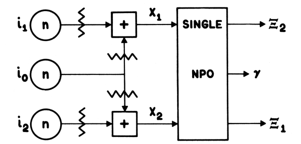
Figure 6—Experimental test configuration for the simulation of an NPO

Obviously, i₀ is an important parameter since it represents the memory relating the spaces X₁ and X₂. Ξ₁ has the property that the magnitude of its projection on i₀ is a maximum while Ξ₂ to the opposite has a zero projection on i₀. γ is the detected version of the eigenvalue of Ch(X₂,X₁).

In the companion paper it was shown how one can provide a Euclidean geometrical representation of the NPO. This representation is shown in Figure 7 which shows the vectors i₀, i₁, i₂, X₁, X₂, Ξ₁, Ξ₂, and the angles Θ₁, Θ₂, and γ. The length of a vector is given by

|X| = κₓ(2πε)⁻¹ᐟ² ∈ H(X)

and the angle between two vectors by

|Θ(X₁,X₂)|-sin⁻¹ ∈ -R(X₁,X₂).

The three vectors i₀, i₁, i₂ provide an orthogonal coordinate system because the corresponding signals are random, i.e.,

κ

R(i₀,i₁,i₂) ≡ 0.

As external observers we have a prior knowledge of this coordinate system; however, the NPO is given only the vectors X₁ and X₂ in the i₀ ⨉ i₁ and i₀ ⨉ i₂ planes. The NPO can reconstruct the entire geometry but the actual output Ξ obviously is constrained to lie in the plane of the input vector X. The following formulas are typical of the relations present.

|Ξ₁|

tan β = ——

|Ξ₂|

cos Θ = cos 2β csc 2γ

cos 2β

cos 2Θ₁ = -1 + 2 ———

1-cos 2γ

cos Θ = cos Θ₁ cos Θ₂.

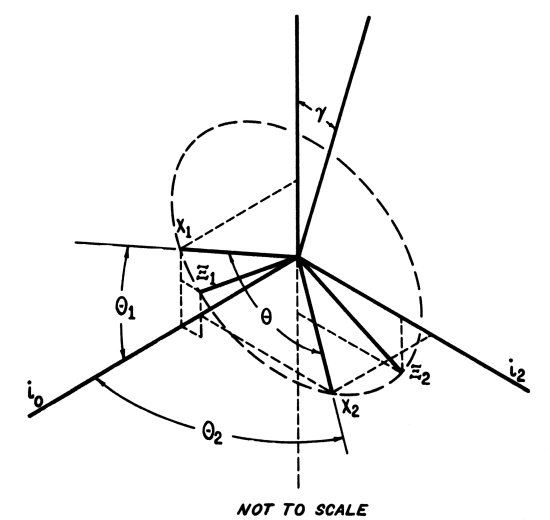
Figure 7—Geometry of the NPO

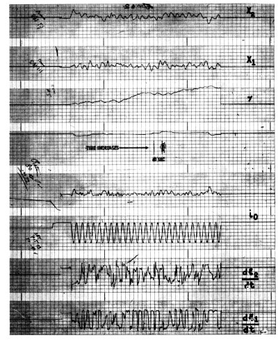
Figure 8—NPO run number 5

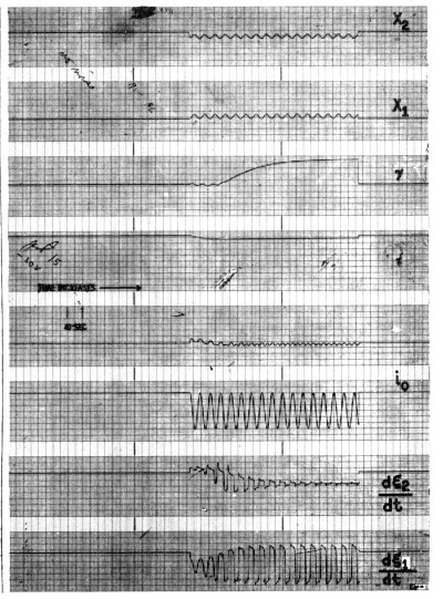
Figure 9—NPO run number 6

We have obtained a complete description of the NPO which involves 74 formulas. These treat the noise in the various outputs, invariances of the NPO and other interesting features. A presentation of these would be outside of the scope of this paper and would tend to obscure the main features of the NPO. Thus, we show here only a typical sample of the computer simulation, Figure 8 and Figure 9. Conditions for these runs are shown in Table I. Run No. 6 duplicates run No. 5 except for the fact that i₁ and i₂ were disabled in run No. 6.

Observe that all our descriptions of the NPO and the space it is to decompose have been time invariant while the signals shown in the simulation are presented as functions of time. The conversion may be effected as follows: Given a measurable (single-valued) function

x = x(t)t ∊ T

where

μ(T) > 0

we define the space

X = {x = x(t) ∍ t ∊ T}

and a probability distribution

μ(x⁻¹(X′))

P(X′) = ———— X′ open ⊂ X

μ(T)

on that space.

TABLE I

Legend for Traces of Figures 8 and 9

Trace Number 1 2 3 4 5 6 7

Symbol X₂ X₁ γ β i dξ₂/dτ dξ₁/dτ

run No. 5

signal 7½ Vrms 7½ Vrms π ptop 35.6 m cps

noise 16 Vrms 15 Vrms π/9 ptop[5] sine wave

DC 0 0

power s/n 1/4 1/4 81/1 0 1/2[6]

terminal value π/4 π/4

run No. 6

signal 7½ Vrms 7½ Vrms π ptop 35.6 m cps

noise 0 0 0[7] sine wave

DC -30V 0

power s/n ∞ ∞ ∞ 0 ∞

terminal value π/4 π/4

Then (X,p(X)) is a stochastic space in our usual sense and x(T) is a stochastic variable. Two immediate consequences are:

P(X) is stationary (P(X) is not a function of t ∊ T), and no question of ergodicity arises.

NETWORKS OF NPO’S

A network of NPO’s may constitute anything from a SOM to a preprogrammed detector, depending upon the relative amount of preprogramming included. Two methods of preprogramming are: (1) Feeding a signal out of a permanent storage into some of the inputs of the network of NPO’s. This a priori copy need not be perfect, because the SOM will measure the angles Θᵢ anyhow. (2) Feedback, which, after all, is just a way of taking advantage of the storage inherent in any delay line. (We implicitly assume that any reasonable physical realization of an NPO will include a delay T between the x input and the ξ output which is not less than perhaps 10⁻¹ times the time constant of the internal feedback loop in the γ computation.)

Simulation of channels that possess a discrete component requires feedback path(s) to generate the required free products of the finitely generated groups. Then, such a SOM converges to a maximal subgroup of the group describing the symmetry of the signal that is a free product available to this SOM.

Because a single NPO with 1 ≤ n₀ ≤ K₀ is isomorphic (provides the same input to output mapping) to a suitable network of NPO’s with n₀ = 1, it suffices to study only networks of NPO’s with n₀ = 1.

Figure 10 is largely self-explanatory. Item a is our schematic symbol for a single NPO with n₀ = 1. Items b, d (including larger feedback loops), and f are typical of artificial intelligence networks. Item c is employed to effect the level changing required in order to apply the three channels in cascade algorithm to the solution of one-dimensional coding problems. Observe that items c and e are the only configurations requiring the γ output. Item d may be used as a limiter by making T⁻¹ high compared to the highest frequency present in the signal. Observe that item e is the only application of NPO’s that requires either the ξ₂ or β outputs. Item f serves the purpose of handling higher power levels into and out of what effectively is a single (larger) NPO.

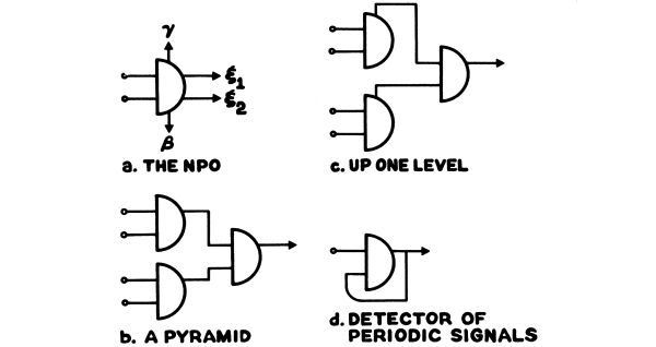
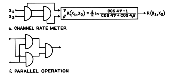
Figure 10—Some possible networks of NPO’s

CONCLUSION

The definition of self-organizing behavior suitably represented has permitted the use of Information Theoretic techniques to synthesize a (mathematical) mechanism for a self-organizing machine. Physical mechanization in the form of an NPO has been accomplished and has introduced the experimental phase of the program. From among the many items deserving of further study we may mention: more economical physical mechanization through introduction of modern technology; identification of networks of NPO’s with their group theoretic descriptions; analysis of the dimensionality of tasks which a SOM might be called on to simulate, and prototype SOM applications to related tasks. It is hoped that progress along these lines can be reported in the future.

REFERENCES

1. Ścibor-Marchocki, Romuald I.,

“A Topological Foundation for Self-Organization,”

Anaheim, California:Northrop Nortronics, NSS Report 2828,

November 14, 1963

2. It is true that our definition is very similar to that proposed by Hawkins (reference 5). Compare for example his definition of learning machines (page 31 of reference 5). But the subsequent developments reviewed therein are different from the one we have followed.

3. Ashby, W. R.,

“The Set Theory of Mechanism and Homeostasis,”

Technical Report 7, University of Illinois,

September 1962

4. Ashby, W. R.,

“Systems and Information,”

Transactions PTGME MIL-7:94-97

(April-July, 1963)

5. Hawkins, J. K.,

“Self-Organizing Systems—A Review and Commentary,”

Proc. IRE. 49:31-48 (January 1961)

6. Mesarovic, M. D.,

“On Self Organizational Systems,”

Spartan Books, pp. 9-36, 1962

7. Braverman, D.,

“Learning Filters for Optimum Pattern Recognition,”

PGIT IT-8:280-285 (July 1962)

8. We make the latter statement despite the fact that we employ a statistical treatment of self-organization. We may predict the performance of, for example, the NPO by using a statistical description, but it does not necessarily follow that the NPO computes statistics.

9. McCulloch, W. S., and Pitts, W.,

“A Logical Calculus of the Ideas Imminent in Nervous Activity,”

Bull-Math. Biophys 5:115 (1943)

10. Newell, A., Shaw, J. C., and Simon, H. A.,

“Empirical Explorations of the Logic Theory Machine:

A Case Study in Heuristic,”

Proc. WJCC, pp. 218-230, 1957

10a. The spaces W, X, Y, and Z are stochastic spaces; that is, each space is defined as the ordered pair (X,p(X)) where p(X) = {p(x) ∋ x ∈ X}, p(x) ≥ 0, x ∈ X and ∫x p(x)dx = 1. Such spaces possess a metrizable topology.

11. We use the following convention for probability distributions: if the arguments of p( ) are different, they are different functions, thus: p(x) ≠ p(y) even if y = x.

12. One can prove the existence of a metric directly but in order to perform the metrization the space has to be decomposed first. But decomposing a space without having a metric calls for a neat trick, accomplished (as far as we know) only by the method used by the SOM.

12a. In this example we use a hemisphere; in general, it would be a spherical cap.