NOTES.

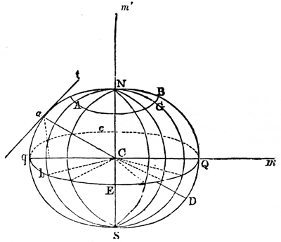
Fig. 1.

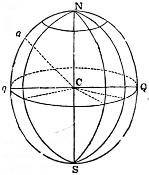
Fig. 2.

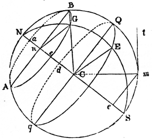
Fig. 3.

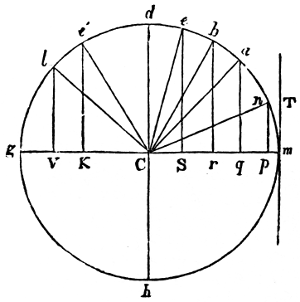
Fig. 4

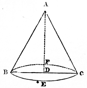
Fig. 5.

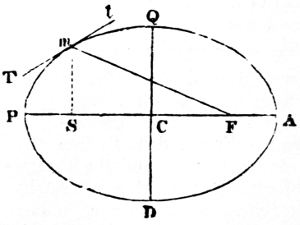
Fig. 6.

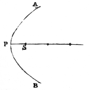
Fig. 7.

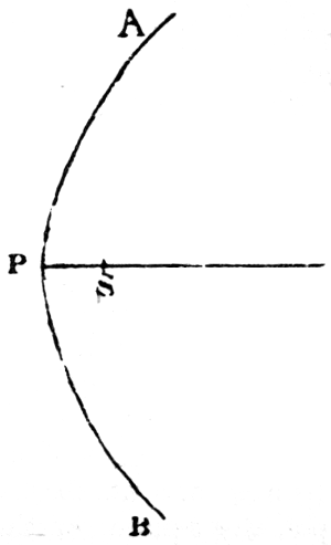
Fig. 8.

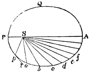
Fig. 9.

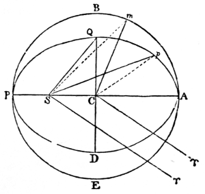
Fig. 10.

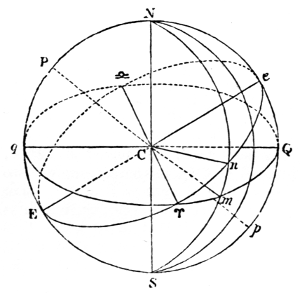
Fig. 11.

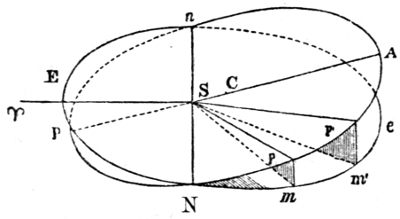
Fig. 12.

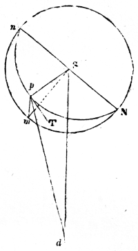
Fig. 13.

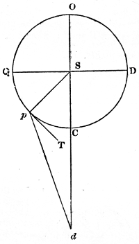
Fig. 14.

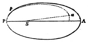
Fig. 15.

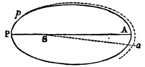
Fig. 16.

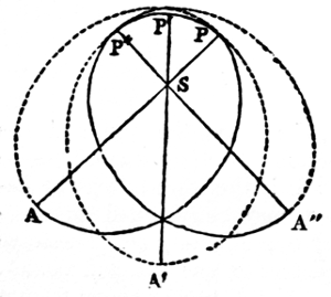
Fig. 17.

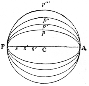
Fig. 18.

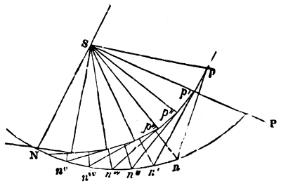
Fig. 19.

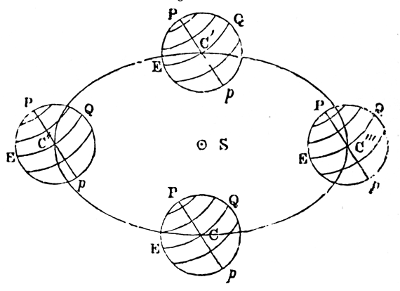
Fig. 20.

Fig. 21.

Fig. 22.

Fig. 23.

Fig. 24.

Fig. 25.

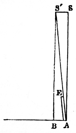
Fig. 26.

To give an idea of the labour requisite merely to perfect or correct the lunar tables, the moon’s place was determined by observation at the Greenwich Observatory in 6000 different points of her orbit, each of which was compared with the same points calculated from Baron Plana’s formulæ, and to do that sixteen computers were constantly employed for eight years. Since the longitude is determined by the motions of the moon, the lunar tables are of the greatest importance.

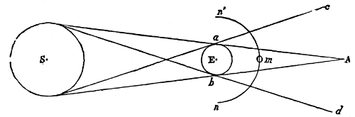
Fig. 27.

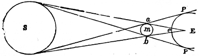
Fig. 28.

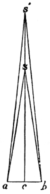
Fig. 29.

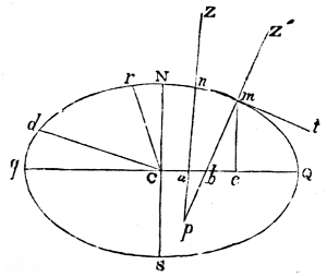
Fig. 30.

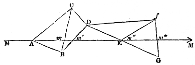
Fig. 31.

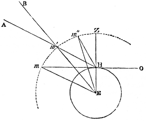
Fig. 32.

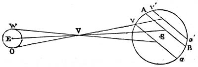
Fig. 33.

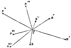
Fig. 34.

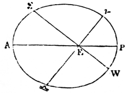
Fig. 35.

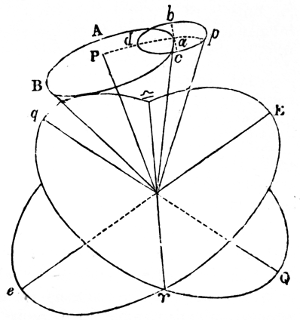
Fig. 36.

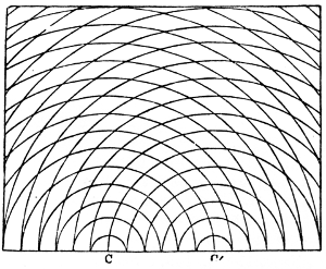
Fig. 37.

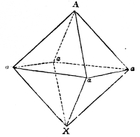
Fig. 38.

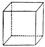
Fig. 39.

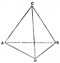
Fig. 40.

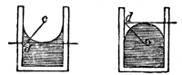
Fig. 41.

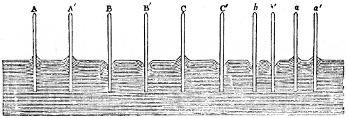
Fig. 42.

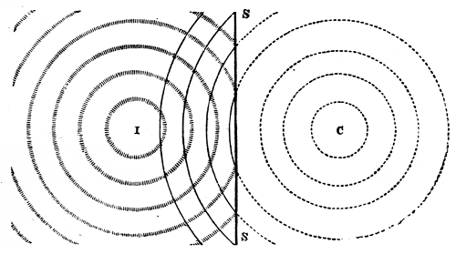
Fig. 43.

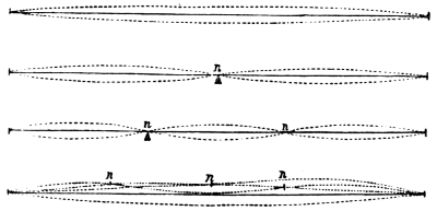
Fig. 44.

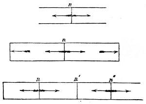
Fig. 45.

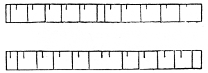
Fig. 46.

Fig. 47.

462

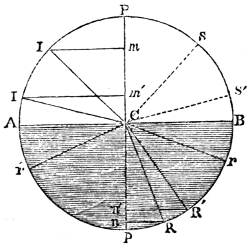
Fig. 48.

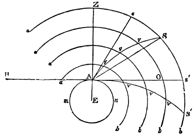
Fig. 49.

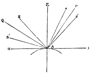
Fig. 50.

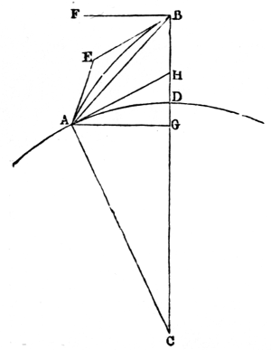
Fig. 51.

465

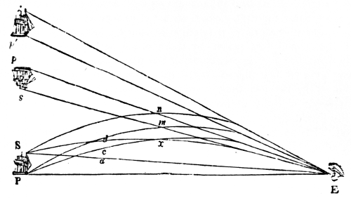
Fig. 52.

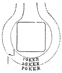
Fig. 53.

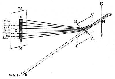
Fig. 54.

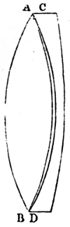
Fig. 55.

(D g V - D g R)/D g G = ·0208/·5362 = 0·03879; for diamond

(D g V - D g R)/D g G = (2·467 - 2·411)/1·439 = 0·0389;

so that the dispersive power of diamond is a little less than that of crown-glass; hence the splendid refracted colours which distinguish diamond from every other precious stone are not owing to its high dispersive power, but to its great mean refraction.—Sir David Brewster.

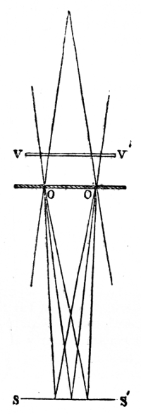
Fig. 56.

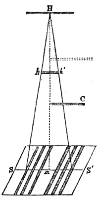
Fig. 57.

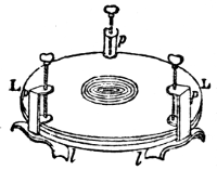
Fig. 58.

1st ring, or 1st order of colours: Black, very faint blue, brilliant white, yellow, orange, red.

2nd ring: Dark purple, or rather violet, blue, a very imperfect yellow green, vivid yellow, crimson red.

3rd ring: Purple, blue, rich grass green, fine yellow, pink, crimson.

4th ring: Dull blueish green, pale yellowish pink, red.

4685th ring: Pale blueish green, white, pink.

6th ring: Pale blue green, pale pink.

7th ring: Very pale blueish green, very pale pink.

After the seventh order the colours become too faint to be distinguished. The rings decrease in breadth, and the colours become more crowded together, as they recede from the centre. When the light is homogeneous, the rings are broadest in the red, and decrease in breadth with every successive colour of the spectrum to the violet.

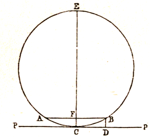
Fig. 59.

1st order: White, pale yellow, yellow, orange, dull red.

2nd order: Violet, blue, whitish, greenish yellow, fine yellow, orange red.

3rd order: Purple, indigo blue, greenish blue, brilliant green, yellow green, red.

4th order: Blueish green, blueish white, red.

5th order: Dull green, faint blueish white, faint red.

4696th order: Very faint green, very faint red.

7th order: A trace of green and red.

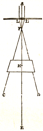
Fig. 60.

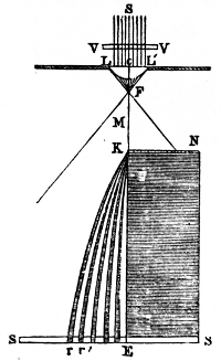
Fig. 61.

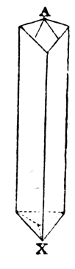
Fig. 62.

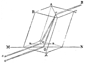
Fig. 63.

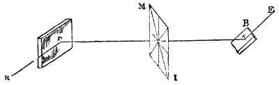
Fig. 64.

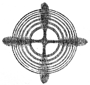
Fig. 65.

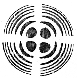
Fig. 66.

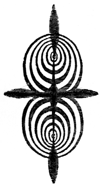
Fig. 67.

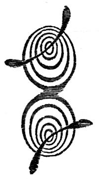
Fig. 68.

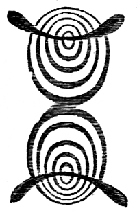
Fig. 69.

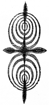
Fig. 70.

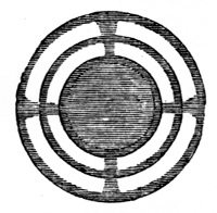
Fig. 71.

474Impetus, vis viva, or living force, is equal to the mass of a body multiplied by the square of the velocity with which it is moving, and is the true measure of work or labour. For if a weight be raised 10 feet, it will require four times the labour to raise an equal weight 40 feet. If both these weights be allowed to descend freely by their gravitation, at the end of their fall their velocities will be as 1 to 2; that is, as the square roots of their heights; but the effect produced will be as their masses multiplied by 1 and 4; but these are the squares of their velocities: hence the impetus or vis viva is as the mass into the square of the velocity.

Thus impetus is the true measure of the labour employed to raise the weights, and of the effect of their descent, and is entirely independent of time. Now heat is proportional to impetus, and impetus is the true measure of labour. In percussion the heat evolved is in proportion to the force of the impetus, and is thus measured by labour.

Travail is a word used in mechanics, to express that work done is equal to the labouring force employed. The work done may be resistance overcome or any other effect produced, while the labouring force may be a horse, a steam-engine, wind, falling water, &c.

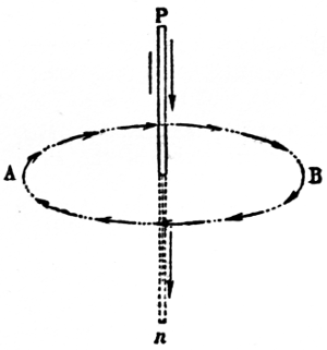
Fig. 72.

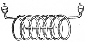
Fig. 73.

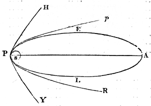
Fig. 74.

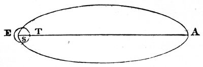
Fig. 75.

Name of Star. Proper Motion. Parallax. Observers and Computers.

α Centauri 3ʺ·764 0ʺ·92 Maclear.

„ .. 1ʺ Henderson.

61 Cygni 5ʺ·123 0ʺ·374 Bessel.

α Lyræ 0ʺ·364 0ʺ·207 Peters.

Sirius 1ʺ·234 0ʺ·230 Henderson.

Arcturus 2ʺ·269 0ʺ·127 Peters.

Pole Star 0ʺ·035 0ʺ·106 Peters.

Capella .. 0ʺ·046 Peters.

La Chevre 0ʺ·461 0ʺ·046 Peters.

ι Great Bear 0ʺ·746 0ʺ·133 Peters.

The space run through in one second by these stars is therefore—

α Centauri 5 leagues Henderson and Maclear.

61 Cygni 10 leagues Bessel.

α Lyræ 2 leagues Struve and Peters.

Sirius 6 leagues Henderson and Maclear.

Arcturus 22 leagues Peters.

Pole Star ½ league Lindenau and Struve.

La Chevre 12 leagues Peters.

ι Great Bear 7 leagues Peters.

There are three great discrepancies in the parallax of the star Argelander or 1830 Groombridge. M. Otto Struve makes it 0ʺ·034, which gives it a velocity of 251 leagues per second, while M. Faye finds the parallax to be between 0ʺ·03 and 0ʺ·01, which makes its velocity from 30 to 85 leagues per second.

These are all minimum velocities, because we can only determine on the celestial vault a projection perhaps much foreshortened of the real motions of the stars.

477

Name of Star. Period in Years. Perihelion Passage. By whom Computed.

ζ Herculis 30·216 1831·41 Madler.

η Coronæ 42·500 1807·21 Madler.

ζ Cancri 58·910 1853·37 Madler.

ξ Ursæ Majoris 58·262 1817·25 Savary.

ω Leonis 82·533 1849·76 Villarceaux.

ρ Ophiuchi 73·862 1806·83 Encke.

3062 in Dorpat Catalogue 94·765 1837·41 Madler.

ξ Bootis 117·140 1779·88 Sir J. Herschel.

δ Cygni 178·700 1862·87 Hind.

γ Virginis 182·120 1836·43 Sir J. Herschel.

Castor 252·660 1855·83 Sir J. Herschel.

ς Coronæ 736·880 1826·48 Hind.

γ Virginis 632·270 1699 Hind.

α Centauri 77·000 1851·50 Jacob.

Orbit of γ Virginis.

Perihelion passage 1836·40

Inclination 27° 36ʹ

Position of ascending Node 19 7

Angle between line of Nodes and Apsides 295° 13

Excentricity 0·8794

Period in years 184·53

Orbit of ζ Herculis.

Perihelion passage 1830·56

Inclination 140° 39ʹ

Position of ascending Node 217° 14ʹ

Angle between line of Nodes and Apsides 266·53

Eccentricity 0·4381

Period in years 37·21

Computed by J. Fletcher, Esq., 1853.

1. An enormous ring seen obliquely with a dark centre and a small star at each extremity.

2. The ring in the constellation Lyra.

3. The dumb-bell nebula in Vulpicula.

4. The spiral nebula or brother system in the 20-feet telescope.

5. A spindle-shaped nebula.

Plate 9 represents some of the same objects as seen by Lord Rosse.

1. Nebula in the girdle of Andromeda.

2. The circular nebula of Lyra.

3. The dumb-bell nebula in Vulpicula.

The spiral nebulæ of 51 Messier, as seen by Lord Rosse, 1 in plate 10, represents fig. 4 of plate 8; and fig. 2 in the same plate is part of the great nebula in Orion, for the whole has never been seen, on account of extreme remoteness.

479