Note 42 — PART SECOND. NOTES ON THE ILLUMINATION OF LIGHTHOUSES, WITH SHORT NOTICES OF THEIR EARLY HISTORY.

See third corollary to Proposition III. of Wallace’s Conic Sections, which shews that a tangent to the parabola makes equal angles with the diameter which passes through the point of contact and a straight line drawn from that point to the focus. The curve may be traced in two different ways, both dependent on the property, that the distance of any point in the parabola from the focus is equal to its distance from the directrix.

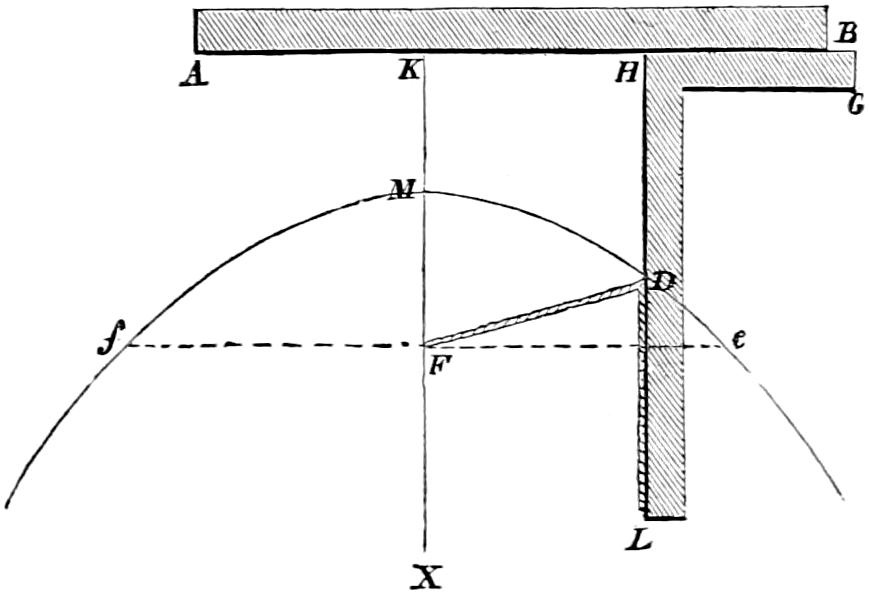
To draw the curve mechanically (fig. 23), let F be the focus, MF the focal distance (chosen at pleasure according to rules which I shall afterwards notice), KMX is the axis, and AB the directrix (the dotted line f F e, bounded by the curve at either end, would then be the parameter or latus rectum). Place the edge of the straight ruler AKHB along the directrix; and let LHB be a square ruler which may slide along the fixed ruler AKHB, so that the edge HL may be constantly perpendicular to AB, or parallel to MX, the axis; let LDF be a string equal in length to HL, and having one end fixed in F, and the other at L, a point in the sliding square. Then if the string be stretched by a pencil D, so as to keep the part DL close to the edge of the square, and if at the same time the square be gently pushed along the line AB, the point D will be forced to move along the edge LH of the square, and will trace out a curve which will be the required parabola. This is obvious from the consideration, that the string LDF being equal in length to LH, and LD being common to both, the remainder DF must be equal to the remainder DH, so that the point which traces the curve being equidistant from the directrix and the focus must, in terms of the above definition, describe a parabola.

Fig. 23.

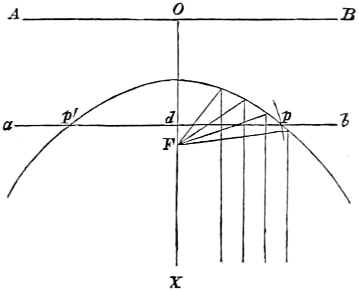
In the second place, the same property, as already stated, furnishes us with the means of tracing the curve by finding successive points therein. Draw a line a b perpendicular to the axis OX, and the position in this line, of a point p through which the curve passes, is easily found thus: Describe from F the focus as a centre with a radius equal to the perpendicular distance O d of the line a b from the directrix AB, a circle cutting the line a b in two points p and p′; then both these points are in the curve. By repeating the same process, any number of points in the curve may be obtained.

Fig. 24.

Lastly, from the equation to the curve, the length y of any ordinate may be computed, in terms of m its principal focal distance, and x its abscissa, by the simple expression,—

y = √4 m x.