LIFE HISTORY

Reproduction

Reproductive activity might have been measured in a number of ways. Three indicators were tested: the percentage of females gravid or lactating, the percentage of juveniles in the month following the sampling period, and the percentage of females with a vaginal orifice in the sampling period. The condition of vagina proved to be most useful. Whether or not there is a vaginal cycle in Microtus is uncertain. Bodenheimer and Sulman (1946:255-256) found no evidence of such a cycle, nor did I in my work with laboratory animals at Lawrence. How much the artificial environment of the laboratory affected these findings is unknown. The presence of an orifice seemed to indicate sexual activity (Hamilton, 1941:9). The percentage of gravid females in the population could not be determined accurately by a live-trapping study and was not useful in this investigation. The percentage of juveniles trapped in the month following the sampling period tended to follow the curve of the percentage of adult females with a vaginal orifice. The ratio of trapped juveniles to adults trapped was a poor indicator of reproductive activity. Juveniles were caught in relatively small numbers because of their restricted movements, and no way to determine prenatal and juvenal mortality was available.

Reproductive activity continues throughout the year. Within the thirty-month period for which data were obtained, December and January showed the lowest percentages of females with vaginal orifices (Fig. 8). The other months all showed higher levels of reproductive activity with a slight peak in the August-September-October period in both 1950 and 1951. In the species of Microtus that are found in the United States, such summer peaks of breeding seem to be the rule (Blair, 1940:151; Gunderson, 1950:17; Hamilton, 1937b:785). Jameson (1947:147) worked in the same county where my field study was made and found that the high point of reproduction was in March, although his samples were too small to be reliable. The peak of reproductive activity slightly preceded the highest level of population density in each year (Fig. 8).

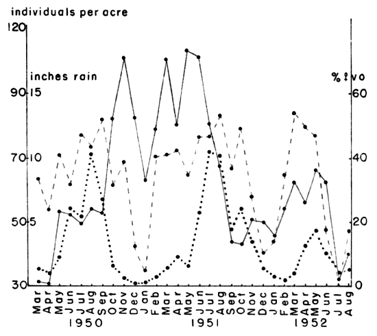
Fig. 8. Variations in density and reproductive rate of voles, with variation in monthly precipitation. Abnormally low rainfall in 1952 caused a decrease in breeding activity and eventually in the numbers of voles. The solid line indicates the number of voles per acre, the broken line the percentage of females with a vaginal orifice and the dotted line the inches of rainfall.

A marked reduction in the percentage of females having vaginal orifices was observed in the unusually dry summer of 1952. The rate of reproduction was found to be positively correlated with rainfall (Fig. 9). Correlation coefficients were higher in each case when the amount of rainfall in the month preceding each sampling period was used instead of that in the month of the sample. This suggested that the rainfall exerted its influence indirectly through its effect on plant growth. Bailey (1924:530) reported that a reduction in either the quantity or quality of food had a depressing effect on reproduction. Drought, such as occurred in 1952, would certainly have a depressing effect on both. The critical factor seems to be the supply of new, actively growing shoots available to the voles for food rather than the total amount of vegetation. As far as could be determined from the small sample of males examined, their fecundity was not affected by rainfall. Some decrease in the percentage of males that were fecund was noted in the winter and was reported also by Jameson (1947:145) but most of the males in any sample were fecund. Thus any depression in the reproductive rate was due to loss of fecundity by females. This was in agreement with reports in the literature on the subject (Baker and Ransom, 1932a:320; 1932b:43).

The correlation coefficient between rainfall and the percentage of adult females with a vaginal orifice was 0.53. This was considered to be surprisingly high in view of the expected effects on the breeding rate of temperature, seasonal diet variations and whatever rhythms were inherent in the voles. When only the summer months were considered the correlation coefficient between rainfall and the percentage of adult females with a vaginal orifice was 0.84. This indicated that, during the season when breeding was at its height, rainfall was a factor in determining the rate of reproduction and when rainfall was scarce, as in the summer of 1952, it seemed to be a limiting factor (Fig. 9).

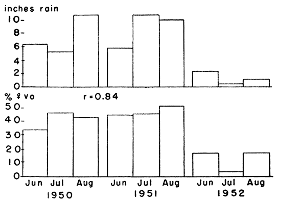
Fig. 9. Comparison between monthly rainfall and reproductive rate of voles in summer. The dry summer of 1952 caused a notable decrease in reproductive activity. The correlation coefficient between rainfall and the percentage of females with a vaginal orifice was 0.84.

Of the total captures 20.6 per cent involved more than one individual. When the distribution of these multiple captures was graphed for the period of study, a high correlation between the percentage of captures that were multiple and the percentage of females with a vaginal orifice (r = 0.70) was found. An even higher correlation (r = 0.76) was observed between the percentage of captures that were multiple and the population density. The higher percentage of multiple captures may have been largely a result of fewer available traps per individual on the area and thus only indirectly related to the rate of reproduction.

Of the multiple captures, 66 per cent involved both sexes. The correlation coefficient between the percentage of captures involving both sexes and the level of reproductive activity was 0.58. Among those pairs of individuals caught together more than once, 61 per cent were composed of both sexes. Among those pairs taken together three or more times 76 per cent were male and female and among those pairs taken together four or more times 80 per cent were male and female. When adult voles stayed together any length of time their relationship usually appeared to be connected with sex. Family groups were also noted, as pairs were often trapped which seemed to be mother and offspring. A lactating female would sometimes enter a trap even after it had been sprung by a juvenile, presumably her offspring, or a juvenal vole would enter a trap after its mother had been captured. Such family groups persisted only until the young voles had been weaned.

The youngest female known to be gravid was 26 days old and weighed 28 grams. During summer most of the females were gravid before they were six weeks old, although females born in October and after were often more than 15 weeks old before they became gravid. The youngest male known to be fecund was approximately six weeks old. Male fecundity was determined as described by Jameson (1950). Difference in the age of attainment of sexual maturity serves to reduce the mating of litter mates (Hamilton, 1941:7) and has been noticed in various species of the genus Microtus by several authors (Bailey, 1924:529; Hatfield, 1935:264; Hamilton, loc. cit.; Leslie and Ransom, 1940:32).

For 35 females, each of which was caught at least once each month for ten consecutive months or longer, the mean number of litters per year was 4.07. Certain of the more productive members of the group produced 11 litters in 16 months. M. ochrogaster seems to be less prolific than M. pennsylvanicus. Bailey (1924:528) reported that one female meadow vole delivered 17 litters in 12 months. Hamilton (1941:14) considered 17 litters per year to be the maximum and stated that in years when the vole population was low the females produced an average of five to six litters per year. In "mouse years" the average rose to eight to ten litters per year. During this study several females delivered two or more litters in rapid succession. This was noted more frequently in spring and early summer than in other parts of the year. Those females which produced two or three litters in rapid succession in spring and early summer often did not litter again until fall. Post-parous copulation has been observed in M. pennsylvanicus by Bailey (1924:528) and Hamilton (1940:429; 1949:259) and probably occurs also in M. ochrogaster.

The gestation period was approximately 21 days, the same as reported for M. pennsylvanicus (Bailey, loc. cit.; Hamilton, 1941:13) and M. californicus (Hatfield, 1935:264). A more precise study of the breeding habits of M. ochrogaster failed to materialize when the voles refused to breed in captivity. Fisher (1945:437) also reported that M. ochrogaster failed to breed in captivity although M. pennsylvanicus (Bailey, 1924) and M. californicus (Hatfield, 1935) reproduced readily in the laboratory.

Litter Size and Weight

In the course of this study 65 litters were observed. The mean number of young per litter was 3.18 ± 0.24 and the median was three (Fig. 10). Three litters contained but one individual and the largest litter contained six individuals. Other investigators have reported the number of young per litter in M. ochrogaster as three or four (Lantz, 1907:18) and 3.4 (1-7) (Jameson, 1947:146). M. pennsylvanicus seems to have larger litters. Although Poiley (1949:317) found the mean size of 416 litters to be only 3.72 ± 0.18, both Bailey (1924:528) and Hamilton (1941:15) found five to be the commonest number of young per litter in that species. Leslie and Ransom (1940:29) reported the average number of live births per litter to be 3.61 in the British vole, M. agrestis. Selle (1928:96) reported the average size of five litters of M. californicus to be 4.8. Hatfield (1935:265), working with the same species, found that litter size varied directly with the age of the female producing the litter. He reported litters of young females as two to four young per litter and of older females as five to seven young per litter. In the litters of M. ochrogaster that I examined, young females did not have more than three young and usually had but two. However, older females had litters of one, two and three often enough so that no relationship, as described above, was indicated clearly.

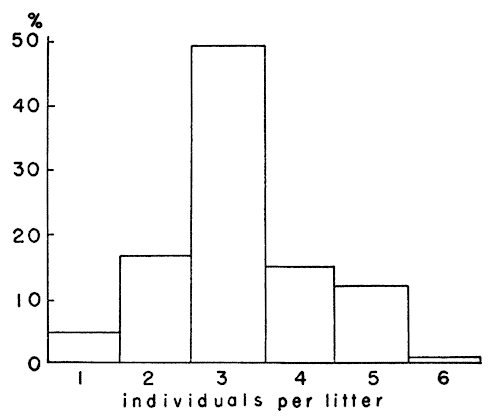
Fig. 10. Distribution of litter size among 65 litters of voles.

No seasonal variation in litter size was noted. The mean size of the litters in 1950, 2.68 ± 0.30, was significantly lower than that found in 1951 (3.76 ± 0.20) but neither differed significantly from the mean size of litters in 1952 (3.35 ± 0.66). The lower mean size of litters was in part coincidental with a high population level and the higher mean of the two later years was in part coincidental with a low population level. Since a sharp break in the curve for population density occurred after the flood in July, 1951, the litters were arranged in pre-flood and post-flood categories for study. Pre-flood litters averaged 3.07 ± 0.28 young per litter whereas post-flood litters averaged 3.34 ± 0.48. This difference was not significant. Increase in litter size, if it had actually occurred, might have been a response to the increasing food supply and lower population density after the flood.

A difference in the mean number of young per litter was noted for those litters delivered in traps as compared with those delivered in captivity and the numbers of embryos examined in the uterus. The mean number of embryos per female was higher than the mean number of young per litter delivered in captivity and the mean number of young per litter delivered in traps was lower than in those delivered in captivity. The differences were not statistically significant. In some instances females that delivered young voles in traps may have delivered others prior to entering the trap or the mother or her trapmates may have eaten some of the newborn voles before they were discovered.

The mean weight of 16 newborn (less than one day old) individuals was 2.8 ± 0.36 grams. No other data on the weight of newborn M. ochrogaster were found in the literature but this mean was close to the 3.0 grams (Bailey, 1924:530) and 2.07 grams (Hamilton, 1937a:504; 1941:10) reported for M. pennsylvanicus and to the 2.7 grams (Selle, 1928:97) and 2.8 grams (Hatfield, 1935:268) reported for M. californicus. No correlation between the weight of the individual newborn vole and the number of voles per litter was observed.

Although the ratio of the average weight of newborn voles to the average weight of an adult female was approximately equal for M. pennsylvanicus and M. ochrogaster, the ratio of the weight of a litter to the average weight of an adult female was larger in the eastern meadow vole because the mean litter size was larger. Perhaps this is related to the more productive habitat in which the eastern meadow vole is ordinarily found.

Size, Growth Rates and Life Spans

The mean weight of adult voles during the period of study was 43.78 grams. The females averaged slightly heavier than the males but the overlapping of weights was so extensive that sexual difference in weight could not be affirmed. The difference observed was less in December and January when gravid females were rare, suggesting that the difference was due, at least in part, to pregnancy. Jameson (1947:128) found, for a sample of 50 voles, a mean weight of 44 grams and a range of 38 to 58 grams. The range in the adult voles I studied was much greater, from 25 to 73 grams. In part, this increase in the range of adult weights was due to a much larger sample.

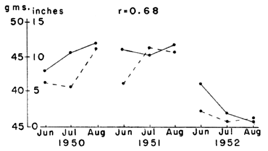
Fig. 11. Relationship between rainfall and the mean weight of adult males in summer. The abnormally low rainfall in the summer of 1952 was accompanied by a decrease in mean weight. The solid line represents mean weight and the broken line rainfall. The correlation coefficient between the two was 0.68.

During the unusually dry summer of 1952, a notable reduction in the mean weight of adults was recorded (Fig. 11). The correlation coefficient between the mean weight of adults and the amount of rainfall for the summer months was 0.68. It seems reasonable to attribute the drop in mean weight to an alteration of plant growth due to decreased rainfall. Some of the reduction in mean weight was due to the loss of weight in older individuals but most of it was due to the failure of voles born in the spring to continue growing.

No data on the growth rate of M. ochrogaster were found in the literature. According to the somewhat scanty data from my study, secured from observations of individuals born in the laboratory, young voles gained approximately 0.6 of a gram per day for the first ten days, approximately one gram per day up to an age of one month, and approximately 0.5 of a gram per day from an age of one month until growth ceases. This growth rate was especially variable after the voles reached an age of thirty days. The growth rate approximates those described for M. pennsylvanicus (Hamilton, 1941:12) and for M. californicus (Hatfield, 1935:269; Selle, 1928:97). Although the data were inadequate for a definite statement, I gained the impression that there was no difference between the sexes in growth rate. In general, young voles grow most rapidly in the April-May-June period and least rapidly in mid-winter. Several voles, born in late autumn, stopped growing while still far short of adult size and lived through the winter without gaining weight, then gained as much as 30 per cent after spring arrived (Fig. 12).

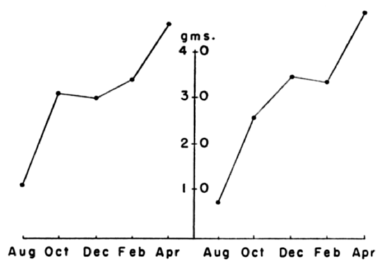
Fig. 12. Growth rates of two voles selected to show typical growth pattern of voles born late in the year. Growth nearly stops in winter and is resumed in spring.

The recorded life spans of most voles studied were less than one year. No accurate mean life span could be determined. Leslie and Ransom (1940:46), Hamilton (1937a:506) and Fisher (1945:436) also found that most voles lived less than one year. Leslie and Ransom (op. cit.: 47) reported a mean life span of 237.59 ± 10.884 days in voles of a laboratory population. In the present study one female was trapped 624 days after first being captured; another female was trapped 617 days after first being captured; and a male was trapped 611 days after first being captured. The two females were subadults when first captured. The male was already an adult when first captured; consequently its life span must have exceeded 650 days. No evidence of any decrease in vigor or fertility was observed to accompany old age.

Of the 45 marked voles snap-trapped in August of 1952, 21 had been captured first as juveniles. The ages of these voles could be estimated within a few days, and the series presented a unique opportunity for studying individual and age variation. Only individuals weighing less than 18 grams when first captured were used, and their ages were estimated according to the growth rate described above. Howell (1924) reported an analysis of individual and age variation in a series of specimens of Microtus montanus, and Hall (1926) studied the changes due to growth in skulls of Otospermophilus grammarus beecheyi. The series of specimens described here differs from those of Hall and Howell, and from any other collection known to me, in the fact that the specimens are of approximately known age and drawn from a wild population.

Unfortunately, this sample was small, and the distribution of the specimens among age groups left much to be desired. No specimens less than one and one-half months old were taken and only a few individuals older than four and one-half months. Table 3 shows the age distribution. The small size of the sample and the absence of juveniles were due, partly, to the unusually dry weather in the summer of 1952. The reduction in the rate of reproduction, caused by drought (as described elsewhere in this paper), reduced the populations and the percentage of juveniles to low levels.

Table 3. Distribution Among Age Groups of 21 Voles Used in the Study of Variation Due to Age

Age in months 1¹⁄₂ 2 2¹⁄₂ 3 3¹⁄₂ 4 4¹⁄₂ 6 12

No. of individuals 1 4 5 1 3 2 3 1 1

In the series of voles studied, ten individuals were in the process of molting from subadult to adult pelage. Jameson (1947:131) reported the molt to occur between eight and 12 weeks of age and selected 38 grams as the lower limit of weight of adults. I also found all voles molting to be between eight and 12 weeks old but found none so large as 38 grams without full adult pelage. This may have been, in part, due to the dry weather delaying or inhibiting growth. Because of the small size of the sample and the influence of the unusual weather conditions, no conclusions concerning normal molting were drawn from the data described below. They are presented only as a description of a small sample drawn from a single population at one time. Table 4 summarizes these data.

Table 4. Mean Sizes and Ages of Voles Molting from Subadult to Adult Pelage

Weight Body length minus tail Condylo-basilar length Age

Six males 32.67 gms. 106.16 mm. 23.78 mm. 9.67 wks.

(30-36) (96-116) (23.2-24.4) (8-12)

Four females 29.0 gms. 100.25 mm. 23.45 mm. 10.5 wks.

(28-30) (98-102) (23.5-23.8) (8-12)

Ten voles 31.2 gms. 103.8 mm. 23.73 mm. 10.0 wks.

(28-36) (96-116) (23.2-24.4) (8-12)

The mean age of the ten voles molting was ten weeks (8-12). Six males averaged 9.67 weeks, almost a week younger than four females, who averaged 10.5 weeks. The difference in age at time of molting between the sexes was not significant. Differences between the sexes in other characteristics to be described also lacked significance. Mean weights at the time of molting were: males, 32.67 gms. (30-36); females, 29.0 gms. (28-30); and all individuals, 31.2 gms. (28-36). Because a piece of the tail of each vole had been removed in marking, the total length of the voles could not be determined. Body length, excluding tail, was used. Howell (1924:986) found this measurement subject to less individual variation than total length and thought body length was probably a better indicator of age. Mean body length at the time of molting was 103.8 mm. (96-116). Males averaged longer than females and were also more variable. The mean body length of males was 106.16 mm. (96-116) and that of females was 100.25 mm. (98-102).

Of the subadults showing no signs of molting, none was above the mean age of molting. Twenty-five per cent of them were longer and heavier than the mean length and weight of those that were molting. Of the 20 adults in the series, one was below the mean weight of molting and one was shorter than the mean length of molting.

When Howell (op. cit.:1014) studied skulls of Microtus montanus he found that the condylobasilar length was the most satisfactory means for arranging his series of specimens according to their age. When the skulls of my series were arranged according to their age (as determined from trapping records) the graph of the condylobasilar lengths showed a clear, though not perfect, relationship to age (Fig. 13). No separation of sexes was made because the sample did not permit it. In Fig. 13 graphs of weight, as determined in the field, and of length (excluding tail) also were included because they are the most easily measured characters of live voles. The graphs indicate individual variation in these characters which limits their usefulness in determining age.

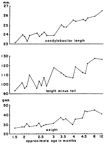
Fig. 13. Graphs of the condylobasilar lengths, body lengths and weights of a series of voles of known age. Within each age group, the youngest vole is on the left in the graphs.

When other cranial measurements, and ratios of pairs of measurements, were plotted in the same order, individual variation obscured some of the variation due to age and the curves resembled those of weight and length of body rather than that of condylobasilar length. When the cranial measurements were averaged for the age groups the curves showed a relationship to age but the relationship of mean measurements is of little use in determining the age of individual specimens. The data described above indicated that a study of the relationship of the condylobasilar length and age in a large sample might provide useful information.

Anyone who has examined mammalian skulls knows of many other characters which vary with age but which are difficult to measure and describe with precision. Figs 14 and 15 are drawings of skulls of voles of known age. The most obvious change, related to aging, evident in the dorsal view of the skulls (Fig. 14) is the increasing prominence and closer approximation of the temporal ridges in older specimens. The lambdoidal ridge is also more prominent in older voles, and their skulls have a generally rougher and more angular appearance. The individual variation evident in these ridges is probably due to variations in the development of the muscles operating the jaws (Howell, 1924:1003). There is an increased flattening of the roof of the skull of older voles.

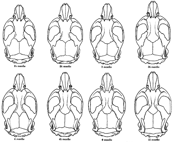
Fig. 14. Dorsal views of skulls of voles of known age. (Ages 1¹⁄₂, 2¹⁄₂, 3, 3¹⁄₂, 4, 4¹⁄₂, 6 and 12 months). All × 3.

View larger image

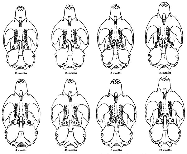
Fig. 15. Palatal views of skulls of voles of known age. (Ages 1¹⁄₂, 2¹⁄₂, 3, 3¹⁄₂, 4, 4¹⁄₂, 6 and 12 months). All × 3.

View larger image

From a palatal view (Fig. 15) the skulls of voles also showed age variation which was apparent but not easily correlated with precise age. The median ridge on the basioccipital bone increases in prominence in older voles. The shape of the posterior margin of the palatine bones changes from a V-shape to a U-shape. On the skull of the oldest (12 months) vole the pterygoid processes are firmly fused to the bullae, a condition not found in any of the other specimens. The anterior spine of the palatine approaches the posterior projection of the premaxillae more closely as age increases and, in the oldest vole is firmly attached and forms a complete partition separating the incisive foramina.

Tooth wear during the life of a vole causes a considerable variation in the enamel patterns, especially of the third upper molar. Howell (1924:1012) considered such variation to be independent of age, but Hinton (1926:103) related the changes to age and interpreted them as a recapitulation of the evolution of microtine molars. In my series, an indentation on the medial margin of the posterior loop of the third upper molar seemed to be related to age. This indentation was absent in the youngest vole (one and one-half months), absent or indefinite in those voles less than 3¹⁄₂ months of age, and progressively more marked in the older voles.

Food Habits

The prairie vole, like other members of the genus Microtus, feeds mostly on growing grass in spring and summer. Piles of cuttings in the runways are characteristic sign of the presence of voles. The voles cut successive sections from the bases of grasses until the young and tender growing tips are within reach. The quantity of grass destroyed is greater than that actually eaten, a fact which will have to be considered in any attempt to evaluate the effects of voles upon a range.

In all piles of cut plants that were examined, Bromus inermis was the most common grass, and Poa pratensis was the grass second in abundance. These were, by far, the most common grasses present on the areas studied; in most places, B. inermis was dominant. Other grasses present on the areas were occasionally found in the piles of cuttings. Jameson (1947:133-136) found no utilization of B. inermis by voles but that grass was present in a relative abundance of only one per cent in the areas studied by him. The voles that he studied ate alfalfa in large amounts and alfalfa was, perhaps, the most common plant on the particular areas where his voles were caught. Seemingly, the diet of voles is determined mostly by the species composition of the habitat.

Other summer foods included pokeberries, blackberries and a few forbs and insects. Forbs most commonly found in the piles of cuttings were the leaves of the giant ragweed (younger plants only) and dandelion. Insect remains were found in the stomachs of voles killed in summer and occurred most frequently in those killed in August and September. At no time did insects seem to be a major part of the diet but they were present in most vole stomachs examined in late summer. Laboratory experiments with summer foods gave inconclusive results but suggested that the voles chose grasses on the basis of their growth stage rather than according to their species. Young and tender grasses were chosen, regardless of species, when various combinations of Triodia flava, Bromus inermis and Poa pratensis were offered to the voles. At times the voles showed a marked preference for dandelion greens, perhaps because of their high moisture content; the voles' water needs were satisfied mostly by eating such succulent vegetation.

Winter foods consisted of stored hay and fruits and of underground plant parts. Bromus inermis made up nearly all of the hay and was stored in lengths of up to ten inches in underground chambers specially constructed for storage. Underground parts of plants were reached by tunnelling and were an especially important part of the voles' diet in January and February. The fruit of Solanum carolinense was eaten throughout the winter and one underground chamber, opened in February, 1952, was packed full of these seemingly unsavory fruits. Fisher (1945:436), in Missouri, found this fruit to be an important part of the winter diet of voles. An occasional pod of the honey locust tree was found partly eaten in a runway. Fitch (1953, in litt.) often observed girdling of honey locust and crab apple (Pyrus ioensis) root crowns on the Reservation but I saw no evidence of bark eating, perhaps because my study plots were mostly grassland. On two occasions when two voles were in the same trap one of them was eaten. In both traps, all of the bait had been eaten and the captured voles probably were approaching starvation. Because the trapping procedure offered abundant opportunity for cannibalism, the low frequency of its occurrence suggested that it was not an important factor in satisfying food requirements under normal conditions.

Runways and Nests

Perhaps the most characteristic sign of the presence of Microtus ochrogaster were their surface runways and underground tunnels. Only rarely was a vole observed to expose itself to full view. When a trapped vole was released it immediately dove out of sight into a runway. Once in a runway, the vole showed no further evidence of alarm and was usually in no hurry to get away. The runways seemed to provide a sense of security and the voles were familiar with their range only through runway travel. The urge to seek a runway immediately when exposed has obvious survival value.

Surface runways were usually under a mat of debris. In areas where debris was scanty or lacking, runways were usually absent. Jameson (1947:136) reported that in alfalfa and clover fields the voles did not make runways as they did in grassland, even in fields where trapping records showed voles to be abundant. Typical surface runways are approximately 50 mm. wide, only slightly cut into the ground and bare of vegetation while in use. Usually they could be distinguished from the runways of the pine vole, which were cut more deeply into the ground, and those of the cotton rat which were wider and not so well cleared of vegetation. Some runways ended in surface chambers and some of these were lined with grass. Their size varied from a diameter of 90 mm. to 250 mm. and they seemed to be used primarily for resting places.

A runway system usually consisted of a long, crooked runway and several branches. Two typical systems are illustrated in Fig. 16. The runway systems often were not clearly limited; they merged with other systems more or less completely. One map showed a runway system extending across 140 square meters and including 12 underground burrows. All of these runways seemed to be part of a single runway system but the system probably was used by more than one vole or family group of voles. Sixteen of the 22 maps that were made extended across areas between 50 and 90 square meters. One map, mentioned above, was larger and the remaining five smaller. The smallest extended across only 20 square meters. Of course, the area encompassed by a set of runways changed almost daily, as the voles extended some runways, added some and abandoned others in the course of their daily travels.

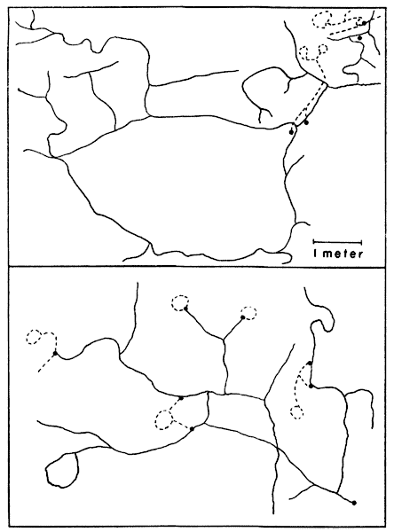
Fig. 16. Maps of runway systems of the prairie vole. The runways follow an irregular course and are frequently changed. The solid lines represent surface runways and the dotted lines underground passages.

Each runway system contained underground nests. These were in chambers from 70 mm. to 200 mm. below the surface and were up to 200 mm. in diameter. Most systems that were mapped had from two to six of these burrows. Most of these were lined with dried grass and seemed to be used for delivering and nursing litters. Each burrow was connected to a surface runway by a tunnel. Often the tunnel was short and the hole opened almost directly into the burrow from the surface runway. Others had tunnels several meters long. Jameson (1947:137) reported every burrow to have two connections with the surface. In the present study, however, I found three arrangements in approximately equal frequency of occurrence: (1) one hole to one tunnel leading to a burrow; (2) two holes to two short tunnels which joined a long tunnel leading to a burrow; and (3) two separate tunnels from the surface to a burrow. The size, depth and number of underground burrows in the systems that I studied varied and so did those reported in the literature. Jameson (loc. cit.) found burrows in eastern Kansas as deep as 18 inches, far deeper than any found in my study. Fisher (1945:435) reported none deeper than five inches in central Missouri. The soil data in my study, as well as in the two reports cited immediately above, were not adequate to permit conclusions, but the type and condition of the soil probably determine the extent of burrowing by the voles of any given locality.

The number of voles using a runway system at one time was difficult to ascertain. In one system, however, four adult individuals were trapped in a ten day period. In August, 1952, at the conclusion of the live-trapping program, a runway system was mapped which had included two trapping stations. In the preceding ten days, four adult voles (three males and one female) had been taken in both traps. During that time, therefore, the runway system was shared by at least four voles. The voles used an area that was considerably larger than that encompassed by any one runway system, a fact obvious when the sizes of home ranges as computed from trapping data were compared with the sizes of the runway systems mapped. A runway system seemed not to be a complete unit, but was only a part of the network of runways used by a single individual.

Activity

Although no special investigation of activity was made, some conclusions concerning it were apparent in the data gathered. There have been a few laboratory studies of the activity pattern of Microtus by various methods. Calhoun (1945:256) reported M. ochrogaster to be mainly nocturnal with activity reaching a peak between dark and midnight and again just before dawn. Davis (1933:235), working with M. agrestis, and Hatfield (1935:263), working with M. californicus, both found voles to be more nocturnal than diurnal. In a field study of M. pennsylvanicus, Hatt (1930:534) found the species to be chiefly nocturnal, although some activity was reported throughout the day. Hamilton (1937c:256-259), however, reported the same species to be more active in the daytime. Agreement on the activity patterns of these species of Microtus has not yet been attained.

From occasional changes in the time of tending a trap line, and from running lines of traps at night a few times in the summer of 1951, I gained the impression that these voles were primarily diurnal. Relatively few of them were caught in the hours of darkness. In summer, however, their activity was mostly limited to the periods between dawn and approximately eight o'clock and between sunset and dark. In colder weather, there was increased activity on sunny days.